STEVE & Subauroral Ion Drift (SAID) Dynamics: How Supersonic Plasma Streams and F-Region Thermal Excitation Forge Radiant Mauve Atmospheric Ribbons
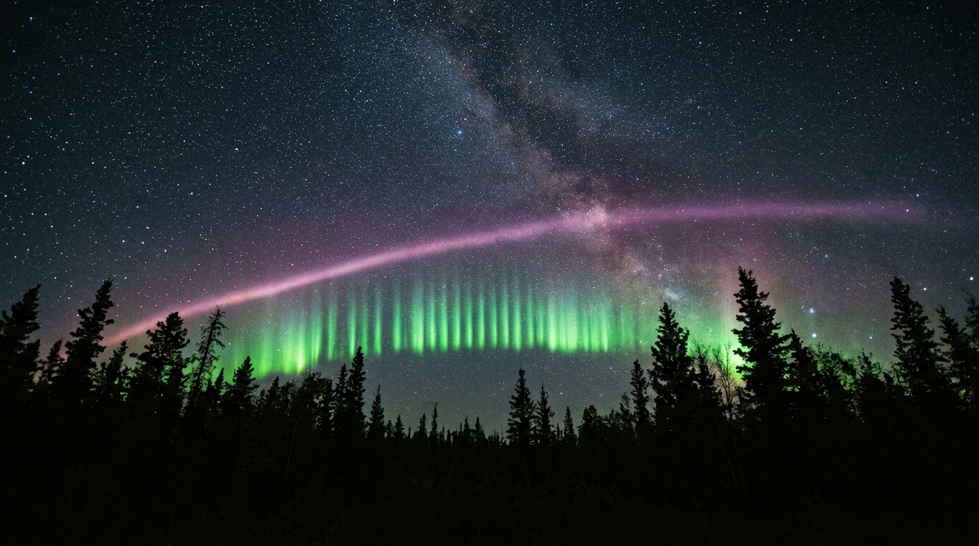
1. Opening Scene
The midnight air across the prairies of central Alberta carries a razor-sharp chill that bites through wool and down. Standing in the open expanse of a darkened farm lane north of Calgary, the stillness of the terrestrial world is absolute. The scent of frost-bitten prairie grass and clean, dry autumn ozone lingers close to the ground, while overhead the celestial sphere unfurls in crystalline clarity. Far to the north, skimming the low horizon, the familiar emerald curtain of the polar aurora borealis ripples quietly—a faint, diffuse luminescence that waxes and wanes against the stars of the Big Dipper.
                           IONOSPHERE (~300-450 km)
        Westward Plasma Drift: v > 5 km/s (Supersonic Stream)
 [West] <==================================================== [East]
        ~~~~~~~~~~~~~~~~~ MAUVE THERMAL EMISSION ~~~~~~~~~~~~~~~~~

             | | | | | | | | | | | | | | | | | | | | | |
             | | | | GREEN PICKET FENCE (100-150 km) | |
             v v v v v v v v v v v v v v v v v v v v v v

        ----------------- GROUND OBSERVER -----------------
Then, without warning, the sky bifurcates. Equatorward of that northern glow, directly overhead in the quiet zenith where traditional auroras almost never venture, a streak of pale mauve light strikes across the dome of the night. It does not cascade or swirl in curtains. Instead, it forms a perfectly straight, razor-thin luminous highway running thousands of kilometres from east to west. As your eyes adapt, the structure intensifies into a vibrant ribbon of lavender and incandescent purple, no wider than two fingers held against the sky. Beneath its southern flank, delicate vertical green fingers—resembling the pickets of a luminous garden fence—flicker and race westward in rhythmic succession. The display is uncanny, motionless in its global alignment yet churning internally with ferocious speed, suspended like a glowing incandescent filament in the deep freeze of the upper atmosphere.
2. What's Actually Happening — Plain English First
To understand why this purple arc astonished the scientific world when it was first documented by the amateur skywatchers of the Alberta Aurora Chasers, one must first grasp how a standard aurora operates.
Think of the upper atmosphere as a massive neon advertising tube. In a classic polar aurora, the sun flings charged particles into Earth’s magnetic embrace. These energetic electrons spiral down the planet’s magnetic field lines and crash into atmospheric gases—predominantly atomic oxygen and molecular nitrogen—around 100 to 200 kilometres above our heads. When an incoming electron strikes an atom, it passes energy to the atom's own electrons, kicking them into an excited state. When those electrons settle back to their resting state, they release that surplus energy as discrete packets of light: vivid emerald green from atomic oxygen, or crimson fringes from nitrogen. The aurora is fundamentally an electrical discharge lamp powered by particle rain.
CONVENTIONAL AURORA (Neon Sign Mechanism)
Incoming Energetic Particles ===> Atomic Excitation ===> Discrete Photon Emission (557.7 nm Green)

STEVE THERMAL EMISSION (Toaster Wire Mechanism)
Supersonic Electric Drift (E x B) ===> Ion-Neutral Friction ===> Extreme Heating (T > 3000 K) ===> Incandescent Glow
The mauve ribbon, officially christened STEVE (Strong Thermal Emission Velocity Enhancement), is not a neon sign. It is an incandescent toaster wire.
When data from citizen scientists were cross-referenced with the European Space Agency Swarm Mission and ground-based all-sky cameras from the NASA THEMIS Mission, physicists realised that satellites crossing this narrow ribbon recorded no heavy rain of energetic particles. Instead, they recorded an extraordinary river of superheated gas: a channel of ionospheric plasma only 25 to 30 kilometres wide, tearing westward at velocities exceeding 5 to 6 kilometres per second—more than 20,000 kilometres per hour.
This hypersonic jet occurs in a subauroral region known to geophysicists as a Subauroral Ion Drift (SAID), embedded within broader Subauroral Polarization Streams (SAPS). As this torrent of charged ions collides with the stationary neutral atmosphere at altitudes between 300 and 450 kilometres, immense friction generates searing thermal energy. The plasma heats up to temperatures exceeding 3,000 to 6,000 Kelvin. Rather than emitting isolated spectral lines, this superheated molecular gas radiates a broad, continuous spectrum of light across multiple wavelengths, blending into the distinctive mauve and purple hue that captivates observers on the ground.
3. The Science (for those who want to go deeper)
The physics governing STEVE bridges magnetospheric convection and ionospheric thermodynamics. When geomagnetic substorms compress and distort Earth’s magnetic tail, powerful voltage potentials build up across the inner boundary of the magnetosphere. In the subauroral ionosphere—an area where electron density drops sharply (the "subauroral trough")—these voltages establish an exceptionally strong poleward electric field ($E_\perp$).
Equation 1: The Electrodynamics of $\mathbf{E} \times \mathbf{B}$ Drift
In any magnetized plasma, the application of a static electric field $\mathbf{E}$ perpendicular to a magnetic field $\mathbf{B}$ exerts a Lorentz force on charged particles. Both ions and electrons gyrate and drift together in a direction perpendicular to both vectors, regardless of their charge sign or mass. This bulk velocity is the $\mathbf{E} \times \mathbf{B}$ drift velocity.
In plain English: The speed of the plasma river is directly proportional to the strength of the electric field squeezing through the magnetic field lines.
$$\mathbf{v}_E = \frac{\mathbf{E} \times \mathbf{B}}{B^2}$$
In scalar terms within the subauroral F-region, where the local geomagnetic field $\mathbf{B}$ points steeply downward into the Northern Hemisphere and the polarization electric field $\mathbf{E}_\perp$ points poleward (northward), the resulting bulk convection velocity $v_d$ is directed westward:
$$v_d = \frac{E_\perp}{B}$$
Worked Example:
Consider satellite instruments traversing an active SAID channel in the F-region ionosphere (approx. 350 km altitude) over central Canada: - Local geomagnetic flux density: $B = 5.0 \times 10^{-5}\text{ T}\ (50\,\mu\text{T})$ - Measured subauroral poleward electric field: $E_\perp = 250\text{ mV/m} = 0.250\text{ V/m}$
Applying the formula: $$v_d = \frac{0.250\text{ V/m}}{5.0 \times 10^{-5}\text{ T}} = 5,000\text{ m/s} = 5.0\text{ km/s}$$
       POLEWARD ELECTRIC FIELD (E_perp ~ 250 mV/m)
                    ^
                    |
                    |
[WEST] <------------+ (v_d ~ 5 km/s)
  Westward Drift    |
                    |
                    X  GEOMAGNETIC FIELD (B ~ 50 uT, Downward into page)
Equation 2: Ion-Neutral Frictional Heating and Thermal Balance
As this stream of positive ions ($\text{O}^+$, $\text{NO}^+$, $\text{O}_2^+$) tears through the background neutral thermosphere composed largely of atomic oxygen ($\text{O}$) and molecular nitrogen ($\text{N}_2$), frequent collisions occur. Because the neutral atmosphere is essentially stationary ($\mathbf{v}_n \approx 0$), this relative velocity dissipates kinetic energy directly into thermal energy via Joule/frictional heating.
In plain English: The temperature of the ions in the stream equals the surrounding air temperature plus an extra boost proportional to the square of their drift speed.
$$T_i = T_n + \frac{m_n}{3 k_B} |\mathbf{v}_i - \mathbf{v}_n|^2$$
Where: - $T_i$ is the effective ion temperature (in Kelvin), - $T_n$ is the background neutral thermospheric temperature ($\sim 1,000\text{ K}$), - $m_n$ is the mean molecular mass of the colliding neutral species, - $k_B$ is the Boltzmann constant ($1.3806 \times 10^{-23}\text{ J}\cdot\text{K}^{-1}$), - $|\mathbf{v}_i - \mathbf{v}_n|$ is the relative drift velocity between ions and neutrals.
Worked Example:
Assuming an F-region background dominated by atomic oxygen ($\text{O}$, atomic weight $16\text{ g/mol}$, so $m_n \approx 2.657 \times 10^{-26}\text{ kg}$), a baseline neutral temperature $T_n = 1,000\text{ K}$, and a measured relative ion drift of $v_i = 5,000\text{ m/s}$:
-
Calculate the frictional temperature increment ($\Delta T$): $$\Delta T = \frac{m_n v_i^2}{3 k_B} = \frac{(2.657 \times 10^{-26}\text{ kg}) \times (5,000\text{ m/s})^2}{3 \times (1.3806 \times 10^{-23}\text{ J/K})}$$ $$\Delta T = \frac{2.657 \times 10^{-26} \times 2.5 \times 10^7}{4.1418 \times 10^{-23}} = \frac{6.6425 \times 10^{-19}}{4.1418 \times 10^{-23}} \approx 16,037\text{ K}$$
-
Account for steady-state collisional cooling and electron coupling: In real ionospheric conditions, while unconstrained ion temperatures can theoretically spike above $10,000\text{ K}$, intense energy transfer to surrounding ambient electrons through Coulomb collisions rapidly elevates the electron temperature ($T_e$) from a baseline of $\sim 1,500\text{ K}$ to sustained levels between $3,000\text{ K}$ and $6,000\text{ K}$.
+-----------------------------------------------------------------------------+
|                      F-REGION THERMAL EQUILIBRIUM                           |
|                                                                             |
|   Supersonic Ion Drift (5 km/s) ---> Ion Frictional Heating (Ti > 8,000 K)  |
|                                                     |                       |
|                                                     v                       |
|   Broad Continuum Emission <--- Electron Heating via Collisions (Te > 3000 K|
+-----------------------------------------------------------------------------+
This superheated electron population transfers energy to molecular nitrogen ($\text{N}_2$) and nitric oxide ($\text{NO}$), exciting vibrational and rotational transitions, alongside radiative continuum processes (such as electron-ion recombination and thermal bremsstrahlung). The absence of a single dominant atomic line means the emitted light spans across the visible spectrum, rendering the macroscopic mauve-purple glow observed from Earth.
The Physics of the "Picket Fence"
The green picket fence presents an intriguing contrast. Spectroscopic analyses confirm that the pickets are pure atomic oxygen emissions at the classical auroral wavelength of $557.7\text{ nm}$ (the forbidden transition $^1\text{S} \rightarrow\ ^1\text{D}$). However, their altitude is much lower—originating in the E-region ionosphere between $100\text{ km}$ and $150\text{ km}$, well beneath the mauve ribbon.
Altitude
 ^
 |  [300-450 km]  MAUVE RIBBON (Thermal Frictional Emission, Te > 3000 K)
 |                =======================================================
 |
 |  [100-150 km]  GREEN PICKET FENCE (Alfvén Waves Accelerate Soft Electrons)
 |                |   |   |   |   |   |   |   |   |   |   |   |   |   |   |
 v                O(1S) -> O(1D) Transition at 557.7 nm
The picket fence is generated by Kinetic Alfvén Waves (KAWs). These electromagnetic plasma waves travel along the steep density gradients at the boundaries of the SAID channel. As they propagate downward into denser atmospheric layers, their parallel electric fields accelerate low-energy "soft" electrons ($\sim 10\text{–}100\text{ eV}$). These electrons selectively excite atomic oxygen at the lower altitude, creating alternating, razor-thin columns of green light aligned precisely along the local geomagnetic field vectors.
4. Practical Outdoor Guidance
Observing STEVE requires distinct strategies from standard auroral chasing. Because STEVE is a transient subauroral phenomenon driven by magnetospheric dynamics, it follows its own geographic and temporal rules.
       GEOMAGNETIC LATITUDE ZONES & OPTIMAL OBSERVATION
+-------------------------------------------------------------+
|  70°N +                                                     |
|       |  POLAR CAP & MAIN AURORAL OVAL                      |
|  65°N |  (Diffuse Green Curtains, Particle Precipitation)   |
|       +-----------------------------------------------------+
|  60°N |                                                     |
|       |  STEVE / SAID OBSERVATION BELT                      |
|  55°N |  (Narrow Mauve Arc + Equatorward Picket Fence)      |
|       +-----------------------------------------------------+
|  50°N |                                                     |
|       |  MID-LATITUDE ZONE                                  |
|  45°N +                                                     |
+-------------------------------------------------------------+
What to Look for in the Sky
- Geomagnetic Latitude ($50^\circ\text{–}60^\circ\text{ N/S}$): Observers located in regions like southern Canada, the northern United States, the United Kingdom, southern Scandinavia, or New Zealand are in prime positions. Unlike conventional auroras that require high latitudes, STEVE appears equatorward of the main auroral oval.
- Morphology and Alignment: Look directly toward the zenith or slightly south of the main auroral display. STEVE manifests as an extremely narrow, continuous ribbon spanning east to west across the entire sky. If you see a broad, wavy green curtain, you are viewing a normal auroral arc. If you see a straight, narrow purple blade cutting overhead from horizon to horizon, you are viewing STEVE.
- Lifespan: STEVE is short-lived. Displays typically persist for only 20 to 60 minutes before fading as the subauroral electric field collapses or neutral drag dampens the ion stream.
Key Space Weather Indicators to Monitor
To anticipate a STEVE event, monitor space weather data provided by the NOAA Space Weather Prediction Center and the Met Office Space Weather Operations Centre: 1. Substorm Recovery Phase: STEVE almost never appears at the onset of a geomagnetic storm. It typically develops during the recovery phase of an intense auroral substorm—approximately 30 to 90 minutes after the primary auroral oval has erupted and begun to recede poleward. 2. Interplanetary Magnetic Field ($B_z$): Watch for a sharp southward turning of the interplanetary magnetic field ($B_z \ll 0$), followed by a sudden northward relaxation. This relaxation triggers the closure of magnetic field lines in the magnetotail, launching the subauroral polarization streams. 3. Ground Magnetometers: Look for significant auroral electrojet index ($AE$ or $AL$) drops exceeding $-500\text{ nT}$ to $-1000\text{ nT}$, followed by a steady upward recovery. Global space weather updates coordinated through the World Meteorological Organization Space Weather Portal provide useful multi-station indices.
Observation Checklist for Skywatchers
| Observation Criterion | Conventional Aurora | STEVE |
|---|---|---|
| Typical Color | Emerald Green ($557.7\text{ nm}$), Crimson ($630.0\text{ nm}$) | Mauve, Violet, Incandescent White, Green Pickets |
| Structure | Wide curtains, undulating rays, pulsating patches | Extremely narrow, straight east-west linear ribbon |
| Sky Position | High-latitude polar sky (toward magnetic pole) | Subauroral zenith ($50^\circ\text{–}60^\circ$ magnetic latitude) |
| Primary Altitude | $100\text{–}200\text{ km}$ | $300\text{–}450\text{ km}$ (Ribbon); $100\text{–}150\text{ km}$ (Pickets) |
| Physical Mechanism | Particle precipitation / atomic excitation | Ion-neutral friction / thermal incandescence + KAWs |
| Duration | Hours (persisting throughout the night) | Brief ($20\text{–}60\text{ minutes}$) |
5. Today's Meteorological Rule of Thumb
When a brilliant northern lights storm begins to calm and recede toward the horizon, do not pack away your camera: look directly overhead into the quiet subauroral sky, where the supersonic thermal ribbon of STEVE is most likely to ignite.