Aurora Borealis & Birkeland Current Dynamics: How Solar Wind-Magnetosphere Coupling and Electron Precipitation Forge Shimmering Polar Curtains
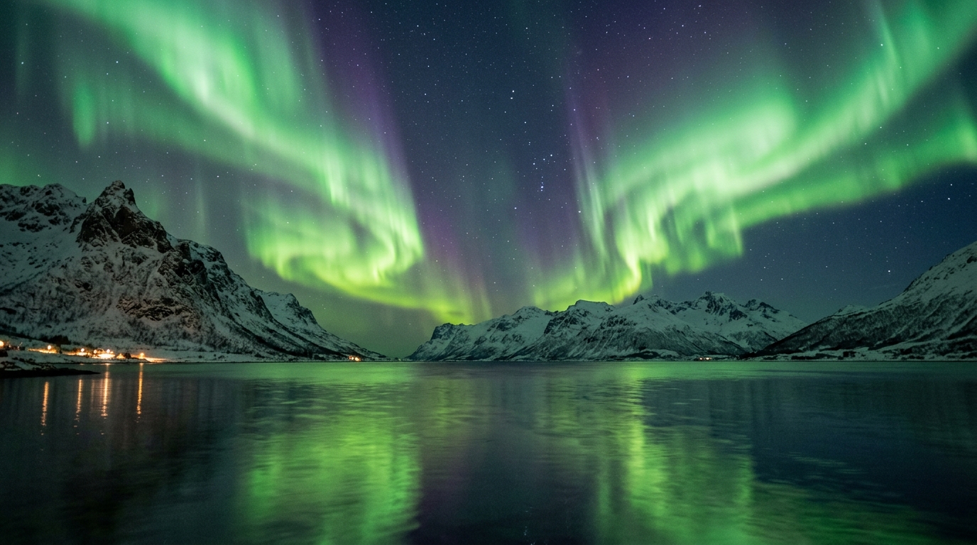
Stand on the windswept expanse of the Finnmark plateau or beside the frozen shores of Lake Torneträsk in Swedish Lapland at two hours past midnight. The air is still, dry, and brutally cold at minus twenty-eight degrees Celsius. Every exhalation crystallises instantly into tiny suspended ice prisms that shimmer faintly under the ambient glow of the winter constellations. There is no wind to stir the snow-laden dwarf birches, yet the atmosphere feels charged with an uncanny, silent tension.
       IONOSPHERE & MAGNETOSPHERIC INTERACTION
             [ Solar Wind: Protons & Electrons ]
                            |
                            v (IMF Bz < 0 Reconnection)
   ==================================================== 400 km
   | Upper Thermosphere: Red Emission [O(1D)]         |
   | 630.0 nm (tau ~ 110 s; quenched below 200 km)     |
   ---------------------------------------------------- 200 km
   | Middle Thermosphere: Green Emission [O(1S)]      |
   | 557.7 nm (tau ~ 0.73 s; 100 - 150 km)            |
   ---------------------------------------------------- 100 km
   | Lower Border: Violet/Magenta [N2+ 1NG Bands]     |
   | 391.4 nm & 427.8 nm (Hard >10 keV Electrons)     |
   ==================================================== 85 km
             [ Earth Surface / Observer ]
On the northern horizon, a faint, pale arc begins to coalesce. To the unadjusted eye, it looks like a wisp of illuminated cirrus cloud, motionless and unassuming. But over several minutes, the arc intensifies, lifting off the horizon and bowing across the magnetic meridian. Its colour resolves into a distinctive, supernatural apple-green.
Without warning, the quiescent arc ruptures into an explosive substorm. Vertical striations—vast parallel flutes of light tens of kilometres tall—ripple from east to west at dozens of kilometres per second. The drapery folds back on itself in complex convolutions, suspended like sheer silk agitated by a cosmic gale. Above the dominant emerald ribbons, the curtains dissolve into a faint, blood-red velvet haze that stretches high toward the zenith. At the lowest edge, where the curtain plunges deepest into the atmosphere, a fleeting fringe of electric magenta and violet flickers. The entire display unfurls in absolute, eerie silence, a grand ballet spanning hundreds of thousands of cubic kilometres of the upper atmosphere, powered by engines millions of miles away in the interplanetary void.
2. What’s Actually Happening — Plain English First
To understand the light show overhead, imagine Earth not as an isolated rock, but as an obstacle sitting in a torrential, supersonic river flowing outward from the Sun: the solar wind. This wind is not air, but a plasma—a searing soup of free electrons and protons racing through space at 400 to 800 kilometres per second, carrying with it the Sun’s own magnetic field, known as the Interplanetary Magnetic Field (IMF).
Earth protects itself with a giant magnetic shield called the magnetosphere. Think of this shield as a teardrop-shaped bubble blown into the solar wind, compressed on the dayside facing the Sun and stretched out behind our planet into a long tail—the magnetotail—that reaches millions of kilometres into the dark of space.
   Solar Wind --->  ( ( [ Dayside Magnetosphere ]
   (IMF Bz < 0)     ( (       |
                    ( (     [Earth] === Birkeland Currents ===> Ionosphere
                    ( (       |
                    ( ( [ Magnetotail: Magnetic Reconnection & Acceleration ]
The crucial trigger for an aurora occurs when the magnetic field carried by the solar wind points southward—the exact opposite direction of Earth’s northward-pointing magnetic field lines at the equator. When two magnetic fields pointing in opposite directions are pressed together, they can violently snap and fuse together in a process called magnetic reconnection.
Think of Earth's magnetic field lines as elastic bands. During reconnection on the dayside, these bands are peeled back by the solar wind and dragged into the nightside tail. As more energy builds up in the tail, the stretched rubber bands suddenly snap back toward Earth. This snapping releases staggering amounts of stored magnetic energy, accelerating clouds of trapped electrons and protons down along Earth's converging magnetic field lines directly into the polar upper atmosphere.
As these energetic particles slam into the upper atmosphere, the mechanism resembles a celestial neon sign. In a neon tube, an electric current excites atoms of gas, which then emit light as they shed that extra energy. In the polar sky, the descending electrons collide with atomic oxygen and molecular nitrogen between 80 and 400 kilometres altitude. Each collision knocks an atmospheric atom or molecule into an "excited" quantum state. When the atom drops back down to its comfortable, resting energy level, it releases that energy as a photon of light whose exact wavelength (and thus colour) is dictated by the quantum mechanics of the specific atom struck.
3. The Science (for those who want to go deeper)
To understand how magnetic energy in deep space transforms into luminous emissions in the upper atmosphere, we must examine the electrodynamics of current systems, the particle mechanics of magnetic confinement, and the quantum radiative kinetics of the upper atmosphere.
3.1 Field-Aligned Currents and Ampère’s Law
The coupling between the distant magnetosphere and the terrestrial ionosphere is mediated by massive electric circuits discovered conceptually by Kristian Birkeland in 1908 and verified by satellite magnetometry in the late 1960s. These are the Birkeland currents (or Field-Aligned Currents (FACs)).
               MAGNETOSPHERE (Generator Region)
                      /              \
     Downward FAC    /                \   Upward FAC
    (Electrons Out) /                  \  (Electrons Precipitating Down)
                   v                    \
            =================================  ~110 km
                   Ionospheric Electrojet
                   (Pedersen/Hall Currents)
During periods of southward IMF ($B_z < 0$), magnetic reconnection establishes a large-scale convective electric field across the magnetotail. This field drives currents of millions of amperes along the helical paths of Earth's geomagnetic field lines directly into the high-latitude ionosphere at roughly $100\text{ to }120\text{ km}$ altitude. In the ionosphere, where collisions with neutrals allow plasma to conduct across magnetic field lines, the circuit closes through the auroral electrojet via Pedersen (parallel to the electric field) and Hall (perpendicular to both $\mathbf{E}$ and $\mathbf{B}$) currents.
The spatial structure of these field-aligned currents can be directly derived from Ampère's Law under magnetohydrodynamic conditions. Because displacement currents are negligible at these low frequencies, the relationship between the magnetic perturbation field $\mathbf{B}$ and the field-aligned current density $\mathbf{J}_\parallel$ is governed by:
$$\nabla \times \mathbf{B} = \mu_0 \mathbf{J}_\parallel$$
Where: * $\nabla \times \mathbf{B}$ is the curl (spatial circulation) of the local magnetic field vector (in $\text{T/m}$). * $\mu_0 = 4\pi \times 10^{-7}\text{ T}\cdot\text{m/A}$ is the permeability of free space. * $\mathbf{J}_\parallel$ is the field-aligned current density (in $\text{A/m}^2$).
Worked Example 1: Calculating Auroral Current Sheet Density
When a research satellite such as the European Space Agency’s Swarm constellation crosses an auroral curtain, its onboard fluxgate magnetometer records a distinct transverse deflection in the magnetic field vector.
Assume an infinite planar current sheet oriented east-west along the auroral oval, with current flowing strictly upward along vertical field lines ($z$-axis). As the satellite flies along the north-south axis ($x$-axis) across the sheet of thickness $\Delta x = 20\text{ km}$ ($2 \times 10^4\text{ m}$), it measures an east-west magnetic field step change $\Delta B_y = 300\text{ nT}$ ($300 \times 10^{-9}\text{ T}$).
Integrating the one-dimensional form of Ampère's Law across the current sheet:
$$\frac{\partial B_y}{\partial x} = \mu_0 J_z \implies J_z = \frac{1}{\mu_0} \frac{\Delta B_y}{\Delta x}$$
Substituting the measured parameters:
$$J_z = \frac{300 \times 10^{-9}\text{ T}}{(4\pi \times 10^{-7}\text{ T}\cdot\text{m/A}) \times (2.0 \times 10^4\text{ m})}$$
$$J_z = \frac{3.0 \times 10^{-7}}{2.513 \times 10^{-2}} \approx 1.19 \times 10^{-5}\text{ A/m}^2 = 11.9\text{ }\mu\text{A/m}^2$$
For an auroral current sheet spanning $3,000\text{ km}$ in longitudinal extent with an integrated linear sheet current density $K = \frac{\Delta B_y}{\mu_0} \approx 0.239\text{ A/m}$, the total integrated upward electric current carried by precipitating auroral electrons exceeds:
$$I_{\text{total}} = K \times L = 0.239\text{ A/m} \times 3.0 \times 10^6\text{ m} \approx 7.17 \times 10^5\text{ A} \approx 0.72\text{ Megamperes}$$
This immense upward current is carried by a downward deluge of thermal and accelerated electrons from the magnetotail, driving the brilliant optical displays monitored by institutions like the British Geological Survey Geomagnetism team.
3.2 The Magnetic Mirror Force and the Loss Cone
Electrons in the magnetosphere do not simply fall under gravity; their trajectories are tightly constrained by the geometry of Earth's dipole magnetic field. As a charged particle spirals along a magnetic field line toward the polar regions, it experiences a converging magnetic field where field lines grow closer together.
Because magnetic forces do no work on charged particles, the total kinetic energy of the electron $E_k = \frac{1}{2}m(v_\parallel^2 + v_\perp^2)$ is conserved. Furthermore, on spatial scales much larger than the particle's gyroradius, the particle's first adiabatic invariant—its magnetic moment $\mu$—remains strictly constant:
$$\mu = \frac{\frac{1}{2} m v_\perp^2}{B} = \frac{E_\perp}{B} = \text{constant}$$
Where: * $E_\perp$ is the kinetic energy associated with motion perpendicular to the magnetic field line. * $B$ is the local magnetic field magnitude.
As an electron travels from the equatorial magnetotail (where $B_{\text{eq}}$ is weak, $\sim 10\text{--}100\text{ nT}$) toward the polar ionosphere (where $B_{\text{iono}}$ is intense, $\sim 50,000\text{ nT}$), $B$ increases by a factor of hundreds. To keep $\mu$ constant, $E_\perp$ must increase proportionally. But because total energy $E_k = E_\parallel + E_\perp$ is fixed, parallel kinetic energy $E_\parallel$ must decrease.
At some critical field strength $B_m$, all parallel energy is converted into perpendicular energy ($E_\parallel = 0$). At this point, the particle reverses its direction along the field line and is reflected back toward the equator. This is the magnetic mirror force:
$$\mathbf{F}\parallel = -\mu \nabla\parallel B$$
   Equatorial Magnetosphere                   Converging Dipole Field
   [ Weak B, Large Pitch Angle ]             [ Strong B near Ionosphere ]
        *                                                \  /
         \                                                \/  Mirror Point (E_parallel = 0)
          \                                               ||  Reflection!
           ~~~~~~~~~~~~~~~~~ Spiral Trajectory ~~~~~~~~~~~||
                                                          /\
                                                         /  \ Loss Cone (Precipitation <150 km)
For an electron to precipitate into the upper atmosphere and cause auroral emissions, its mirror altitude must lie below the dense thermosphere ($<200\text{ km}$). The range of initial equatorial pitch angles $\alpha_{\text{eq}} = \arctan(v_\perp / v_\parallel)$ that allows a particle to reach the atmosphere defines the loss cone, governed by:
$$\sin^2 \alpha_c = \frac{B_{\text{eq}}}{B_{\text{iono}}}$$
Worked Example 2: Determining the Loss Cone Pitch Angle
Consider an electron residing in the plasma sheet at an equatorial distance of $L = 6.6$ Earth radii (geostationary orbit). At this location, the equatorial magnetic field strength is $B_{\text{eq}} \approx 110\text{ nT}$. The magnetic field at the footpoint of this field line in the auroral ionosphere at $100\text{ km}$ altitude is $B_{\text{iono}} \approx 55,000\text{ nT}$.
We can calculate the critical equatorial pitch angle $\alpha_c$ below which the electron will escape magnetic mirroring and precipitate into the atmosphere:
$$\sin^2 \alpha_c = \frac{110\text{ nT}}{55,000\text{ nT}} = \frac{1}{500} = 0.0020$$
$$\sin \alpha_c = \sqrt{0.0020} \approx 0.04472$$
$$\alpha_c = \arcsin(0.04472) \approx 2.56^\circ$$
Only electrons whose initial velocities lie within an extremely narrow cone of roughly $2.6^\circ$ around the magnetic field vector will hit the atmosphere naturally.
To sustain a bright, hours-long auroral substorm, wave-particle interactions—specifically resonant scattering by whistler-mode chorus waves and electrostatic electron cyclotron waves—must continuously scatter trapped electrons, knocking their pitch angles into the loss cone at rates approaching the theoretical limit of strong diffusion.
3.3 Quantum De-excitation, Collisional Quenching, and Altitude Stratification
Once electrons cross the loss-cone threshold and enter the thermosphere, they undergo inelastic collisions with atmospheric constituents. The spectral architecture of the aurora borealis is dictated by the electronic configuration of atomic oxygen ($\text{O}$) and molecular nitrogen ($\text{N}_2$), combined with the barometric decrease in atmospheric density.
       ATOMIC OXYGEN ENERGY LEVELS & EMISSION TRANSITIONS

       Energy (eV)
         4.19 eV  ------------------------ 1S State
                  |                      |
                  |                      | (tau ~ 0.73 s)
                  | (Cascade)            |  ===> 557.7 nm (Emerald Green)
                  |                      |
         1.97 eV  ------------------------ 1D State
                  |
                  | (tau ~ 110 s)
                  |  ===> 630.0 nm / 636.4 nm (Crimson Red)
                  |       [Quenched by N2 below 200 km]
                  |
         0.00 eV  ------------------------ 3P Ground State (Triplet)
The probability of an excited state undergoing spontaneous radiative de-excitation is given by the Einstein $A$-coefficient $A_{ik}$ (in units of $\text{s}^{-1}$). The intrinsic radiative lifetime $\tau$ of an excited state is:
$$\tau = \frac{1}{\sum_k A_{ik}}$$
However, in a dense gas, an excited atom can also lose its energy non-radiatively via collisions with surrounding molecules (primarily $\text{N}_2$) before it has time to emit a photon. This process is known as collisional quenching.
The effective quantum yield $\eta$ (the ratio of emitted photons to initial excitations) is expressed by the Stern-Volmer relationship:
$$\eta = \frac{A_{ik}}{A_{\text{total}} + \sum_j k_j [M_j]}$$
Where: * $k_j$ is the rate coefficient for quenching by species $j$ (in $\text{cm}^3/\text{s}$). * $[M_j]$ is the number density of the quenching species (in $\text{cm}^{-3}$).
1. The Emerald Green Line: $\text{O}(^1S) \to \text{O}(^1D)$ at $557.7\text{ nm}$
- Transition: Atomic oxygen in the metastable singlet-$S$ ($^1S$) state decaying to the singlet-$D$ ($^1D$) state.
- Radiative Lifetime: $\tau \approx 0.73\text{ seconds}$ ($A \approx 1.37\text{ s}^{-1}$).
- Altitude Domain: $100\text{ to }150\text{ km}$.
- Mechanism: Incoming auroral electrons with kinetic energies of $1\text{ to }10\text{ keV}$ penetrate deeply into the thermosphere, colliding with ground-state atomic oxygen: $$e^- + \text{O}(^3P) \to e^- + \text{O}(^1S)$$ Because the radiative lifetime is short ($\sim 0.73\text{ s}$), the de-excitation occurs before collisional quenching can dominate at altitudes above $100\text{ km}$. The resulting $557.7\text{ nm}$ photon falls precisely within the peak photopic sensitivity curve of the human eye, producing the classic green hue that defines most auroral displays.
2. The High-Altitude Crimson Red Line: $\text{O}(^1D) \to \text{O}(^3P)$ at $630.0\text{ nm}$ / $636.4\text{ nm}$
- Transition: Atomic oxygen decaying from the singlet-$D$ ($^1D$) state to the ground triplet-$P$ ($^3P$) state.
- Radiative Lifetime: $\tau \approx 110\text{ seconds}$ ($A \approx 9.1 \times 10^{-3}\text{ s}^{-1}$). This is a spin-forbidden, electric-quadrupole transition.
- Altitude Domain: $200\text{ to }400\text{ km}$.
- Mechanism & Quenching: Because $\tau \approx 110\text{ s}$, an excited $\text{O}(^1D)$ atom must remain undisturbed for nearly two minutes to emit its $630.0\text{ nm}$ photon. Below $200\text{ km}$, the molecular nitrogen density $[N_2] > 10^{10}\text{ cm}^{-3}$ is so high that the mean time between collisions is less than a second.
The atom transfers its energy into vibrational modes of nitrogen: $$\text{O}(^1D) + \text{N}_2 \to \text{O}(^3P) + \text{N}_2(\nu > 0)$$ This reaction quenches the red emission completely in the lower thermosphere. Only above $200\text{ km}$, where the atmospheric density drops below $10^9\text{ cm}^{-3}$, can $\text{O}(^1D)$ survive long enough to radiate spontaneously, producing the soft, diffuse red crowns observed at high altitudes during intense geomagnetic storms.
3. The Low-Border Violet and Magenta Fringe: $\text{N}_2^+$ First Negative Group ($391.4\text{ nm}$, $427.8\text{ nm}$)
- Transition: Ionised molecular nitrogen in the $B^2\Sigma_u^+$ excited state transitioning to the ground ionic state $X^2\Sigma_g^+$: $$\text{N}_2^+(B^2\Sigma_u^+) \to \text{N}_2^+(X^2\Sigma_g^+) + h\nu$$
- Radiative Lifetime: $\tau \approx 60\text{ nanoseconds}$ ($6.0 \times 10^{-8}\text{ s}$).
- Altitude Domain: $85\text{ to }100\text{ km}$.
- Mechanism: This is an allowed dipole transition with an extremely fast decay rate. It requires highly energetic, "hard" electrons ($>10\text{ to }30\text{ keV}$) capable of penetrating down past $100\text{ km}$ into the dense nitrogen-rich mesopause before stopping. The resulting intense violet ($391.4\text{ nm}$) and blue ($427.8\text{ nm}$) emissions combine visually with the lower-altitude green light to produce an electric pink, magenta, or crimson lower border on fast-moving curtains.
Spectral and Physical Characteristics of Auroral Emissions
- $630.0\text{ nm} / 636.4\text{ nm}$ (Deep Red): Emitter: $\text{O}(^1D)$; Lifetime: $\sim 110\text{ s}$; Altitude: $200\text{--}400\text{ km}$; Energy threshold: $\sim 1.97\text{ eV}$; Quenched by $\text{N}_2$ collisions below $200\text{ km}$.
- $557.7\text{ nm}$ (Emerald Green): Emitter: $\text{O}(^1S)$; Lifetime: $0.73\text{ s}$; Altitude: $100\text{--}150\text{ km}$; Energy threshold: $\sim 4.19\text{ eV}$; Dominant photopic emission line.
- $391.4\text{ nm} / 427.8\text{ nm}$ (Violet/Blue): Emitter: $\text{N}_2^+(B^2\Sigma_u^+)$; Lifetime: $\sim 60\text{ ns}$; Altitude: $85\text{--}100\text{ km}$; Requires hard precipitating electrons ($E > 15\text{ keV}$).
- First Positive Bands (Pink/Red): Emitter: $\text{N}_2(B^3\Pi_g \to A^3\Sigma_u^+)$; Lifetime: $\sim 6\text{ }\mu\text{s}$; Altitude: $80\text{--}90\text{ km}$; Fast permitted molecular bands at the lowest auroral fringes.
4. Practical Outdoor Guidance
Chasing and observing the aurora borealis requires monitoring real-time telemetry from deep-space satellites and understanding local geophysical conditions. Real-time solar wind data is continuously collected by the DSCOVR and ACE spacecraft stationed at the Sun-Earth Lagrange Point 1 (L1), roughly 1.5 million kilometres upstream of Earth, providing a 30- to 60-minute advance warning before solar wind structures impact the magnetosphere.
  Upstream L1 (ACE / DSCOVR) === 1.5M km ===> Earth Magnetosphere
  [ Measures Bz, V_sw, Density ]              [ Geomagnetic Response ]
  Data Delay: 30 - 60 minutes                  [ Kp Index, Auroral Oval ]
What to Track on Space Weather Dashboards
When evaluating live data from services like the NOAA Space Weather Prediction Center (SWPC) or the Met Office Space Weather Operations Centre, focus on these four core metrics:
- Interplanetary Magnetic Field Vector ($B_z$ in GSM Coordinates): * The single most critical parameter. For significant auroral activity, $B_z$ must be oriented southward (negative). * A steady $B_z \le -5\text{ nT}$ signals moderate activity; $B_z \le -10\text{ nT}$ to $-25\text{ nT}$ indicates a severe geomagnetic storm. If $B_z$ is strongly positive (northward), the dayside magnetosphere remains closed, and the aurora will usually stall as a faint, stationary arc regardless of solar wind speed.
- Solar Wind Velocity ($v_{\text{sw}}$): * Ambient solar wind speeds average $300\text{ to }400\text{ km/s}$. Coronal Hole High-Speed Streams (CH HSS) or Coronal Mass Ejection (CME) shock fronts elevate speeds to $600\text{--}900+\text{ km/s}$. Higher velocities multiply the rate of magnetic flux transfer into the magnetotail.
- Solar Wind Dynamic Pressure ($P_{\text{dyn}}$): * Dynamic pressure measures the momentum transfer of the solar wind, calculated as: $$P_{\text{dyn}} = \rho v_{\text{sw}}^2 = n_p m_p v_{\text{sw}}^2$$ (where $n_p$ is proton density in $\text{m}^{-3}$ and $m_p = 1.673 \times 10^{-27}\text{ kg}$). * Normal values range from $1\text{ to }3\text{ nPa}$. Sudden pressure spikes exceeding $5\text{ to }20\text{ nPa}$ compress the magnetopause from its normal standoff distance of $10\text{ }R_E$ down to $<6.6\text{ }R_E$, triggering sudden storm commencements (SSCs).
- Planetary $Kp$ Index and Hemispheric Power (HP): * The $Kp$ index is a quasi-logarithmic scale from $0$ to $9$ derived from sub-auroral ground magnetometers worldwide over 3-hour intervals. A $Kp$ of $0\text{ to }2$ confines auroras to Arctic latitudes ($>67^\circ\text{ N}$). $Kp \ge 5$ (G1 storm) pushes the oval south toward Scotland and the northern US border. $Kp \ge 8\text{ or }9$ (G4–G5 storms) allows observers in southern England, central Europe, and the mid-latitude US to witness active displays overhead. * Hemispheric Power (HP), measured in gigawatts ($\text{GW}$) via polar-orbiting satellites, gives an instantaneous estimate of the total auroral energy input: $>20\text{ GW}$ indicates unsettled conditions, while $>100\text{ GW}$ denotes a major auroral substorm.
       GEOMAGNETIC ACTIVITY TIERS & OBSERVATION LATITUDES
 ----------------------------------------------------------------------
  Kp Index   Storm Level   Hemispheric Power   Equatorward Visibility
 ----------------------------------------------------------------------
  Kp 0 - 2   Quiet         < 20 GW             Tromsø, Fairbanks (>66° N)
  Kp 3 - 4   Unsettled     20 - 50 GW          Trondheim, Reykjavik (63° N)
  Kp 5 - 6   G1 - G2 Minor 50 - 100 GW         Edinburgh, Oslo, Calgary (55° N)
  Kp 7 - 8   G3 - G4 Major 100 - 200 GW        Manchester, Seattle, Chicago (50° N)
  Kp 9       G5 Extreme    > 200 GW            London, Paris, Central US (<45° N)
 ----------------------------------------------------------------------
Ground Observation Guidelines
- Target Magnetic Midnight: The peak probability of dynamic auroral substorms occurs around magnetic midnight—the moment when the observer's location is aligned directly opposite the Sun along Earth's magnetic dipole axis. Depending on your geographic longitude and magnetic declination, this typically falls between 23:00 and 01:30 local standard time.
- Allow Complete Dark Adaptation: The human eye relies on scotopic (rod-dominated) vision to detect low-intensity emissions. Rod cells are insensitive to the long-wavelength red line ($630.0\text{ nm}$) and require 20 to 30 minutes of uninterrupted darkness to reach maximum chemical sensitivity (rhodopsin accumulation). Avoid looking at smartphone screens without a physical red filter.
- Monitor Local Ground Magnetometers: Modern skywatchers can track real-time variometer plots from networks operated by the World Meteorological Organization (WMO) or national geological surveys. A sharp downward deflection in the horizontal magnetic component ($H$-trace) of more than $300\text{ to }1,000\text{ nT}$ indicates that an auroral electrojet has formed directly overhead, signalling an imminent substorm breakup within minutes.
5. Today's Meteorological Rule of Thumb
The Auroral Triad Rule: When the interplanetary magnetic field locks southward ($B_z \le -5\text{ nT}$) for more than forty-five minutes while solar wind velocity exceeds $500\text{ km/s}$, an auroral substorm is inevitable. Look toward your magnetic pole within one hour of magnetic midnight: if the lower border shifts from emerald green to a sharp magenta-violet fringe, hard electrons are penetrating below $100\text{ km}$, and the substorm is reaching its energetic peak.