Twomey Effect & Cloud Albedo Dynamics: How Aerosol Influxes and Droplet Sizing Brighten Tropospheric Cloud Decks

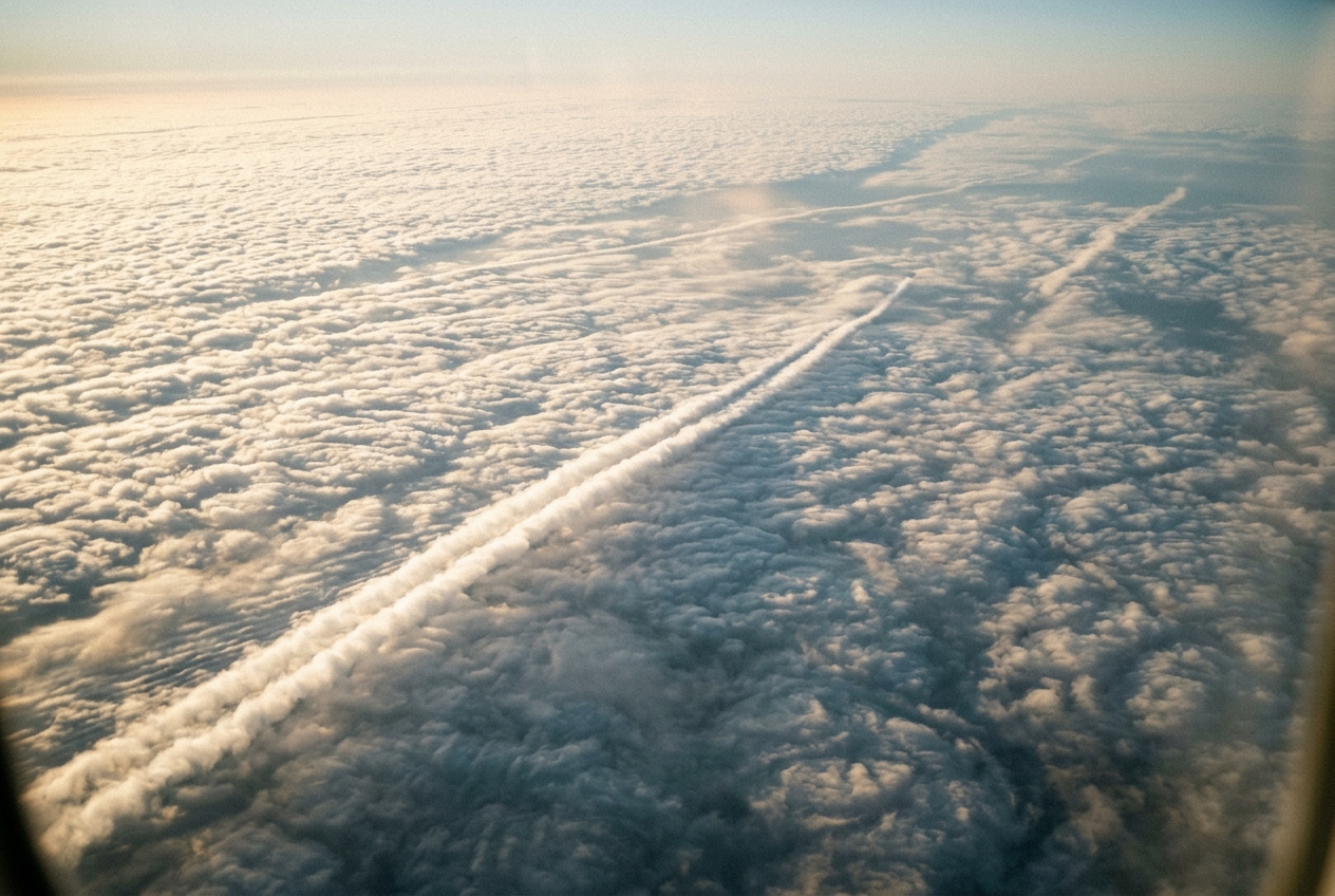
Cruising above the eastern Pacific marine boundary layer, the unbroken grey blanket of stratocumulus reveals brilliant ribbons of reflected sunlight. Here lies the signature of the Twomey effect—where aerosol emissions fundamentally alter cloud optics and the global radiation budget.

1. Opening Scene: The Brilliant Scars Across the Marine Stratocumulus

Stand upon the wind-battered headlands of Point Reyes, California, or gaze through the cockpit window of an atmospheric research aircraft cruising at two thousand metres above the subtropical eastern Pacific. Below, a continuous, undulating deck of marine stratocumulus spreads to the horizon like a vast, corrugated field of fleece. The ocean below is entirely hidden beneath this boundary-layer roof, trapped beneath a sharp thermal inversion where warm, dry tropospheric air caps the cool, humid maritime boundary layer.

In pristine air, this marine cloud deck presents a soft, matte pearl-grey appearance. The ambient air feels intensely clean, carrying the saline, mineral tang of sea spray and ozone whipped up by steady northwesterly trades. The barometric pressure sits steady, while the relative humidity at the surface hovers near 90 percent. As you look out across the expanse of clouds, your eyes are suddenly arrested by vivid, razor-sharp ribbons of dazzling white inscribed across the overcast canvas.

Solar Irradiance (F_0)
       \   \   \   \
        v   v   v   v
  =================================  <-- Cloud Top Inversion
  [ Pristine: r_e ≈ 12 µm, N ≈ 50 ]  --> Forward scattering / Darker (A ≈ 0.50)
  ---------------------------------
  [ Ship Track: r_e ≈ 6 µm, N ≈ 400] --> Enhanced backscatter / Bright (A ≈ 0.67)
  =================================
             Ocean Surface (Dark, Albedo ≈ 0.06)

These brilliant lanes—often hundreds of kilometres long and several kilometres wide—are not gaps in the cloud deck, nor are they elevated plumes of steam. They are ship tracks: enduring microphysical modifications embedded directly within the cloud layer, traced along the invisible shipping lanes that link the Pacific Rim.

Inside these tracks, the cloud does not contain more liquid water than its surroundings; in fact, the total mass of condensed moisture remains nearly identical across the boundary. Yet, beneath the midday sun, these narrow corridors reflect incoming solar radiation with an intensity that outshines the ambient deck by tens of percentage points.

Downwind of major coastal industrial zones, an identical phenomenon unfolds on a regional scale. When continental plumes laden with combustion particles drift offshore over the dark ocean, entire cloud fields undergo an abrupt optical transformation, turning from subdued, translucent grey sheets into brilliant, blinding reflectors of shortwave sunlight.

2. What's Actually Happening — Plain English First

To understand why a cloud suddenly brightens without gaining any extra water, consider how light interacts with matter. Cloud droplets do not produce their own illumination; they act as microscopic spherical mirrors and prisms that intercept incoming sunlight, scattering individual photons in all directions.

Think of the liquid water in a cloud as a fixed lump of baker’s dough. If you leave that dough as a single large loaf, it has a modest surface area. But if you divide that exact same volume of dough into hundreds of bite-sized rolls, the total surface area exposed to the air multiplies dramatically.

In the atmosphere, liquid water cannot condense out of thin air on its own under ordinary supersaturations; water vapour requires microscopic airborne seeds known as Cloud Condensation Nuclei (CCN).

In the pristine maritime boundary layer, far from human activity, these nuclei are scarce. The atmosphere might contain only 50 to 100 condensation nuclei per cubic centimetre, primarily composed of naturally occurring sea salt crystals and biogenic sulfate particles released by ocean phytoplankton. When an air parcel rises, cools, and reaches its dew point, the available water vapour condenses onto this small population of seeds. The resulting droplets grow large—often 10 to 15 micrometres in radius—creating a cloud populated by relatively few, large water spheres.

When a container ship steams beneath the cloud deck or an industrial coastal city vents its exhaust into the marine layer, billions of microscopic combustion aerosols (sulfates, nitrates, and unburnt organic carbon) are injected into the boundary layer. These particles act as highly efficient cloud condensation nuclei.

When the next convective updraft occurs, the exact same quantity of ambient water vapour is now distributed across 500 to 1,000 nuclei per cubic centimetre. Because the available water is partitioned among ten times as many condensation centres, the droplets are starved of volume and remain much smaller—often only 4 to 6 micrometres in radius.

Because scattering occurs at the surface of the droplets, multiplying the number of small droplets dramatically expands the aggregate cross-sectional surface area of water within the cloud. Incoming solar photons encounter far more droplet surfaces per metre of descent through the cloud deck.

Instead of penetrating deep into the cloud or passing through to the dark ocean below, photons undergo multiple scattering events near the cloud top and are bounced back upward into space. This physical mechanism is known to atmospheric scientists as the Twomey effect (or the first aerosol indirect radiative effect), first quantified mathematically by cloud physicist Sean Twomey in 1977.

3. The Science (for those who want to go deeper)

To understand cloud albedo dynamics and aerosol-cloud interactions quantitatively, we must follow the mathematical bridge connecting microscopic droplet thermodynamics to macroscopic radiative transfer.

Microphysical Scaling: Droplet Concentration and Effective Radius

We begin with the fundamental definition of the Liquid Water Content ($\mathrm{LWC}$), which represents the mass of condensed liquid water per unit volume of air (typically expressed in $\text{g m}^{-3}$ or $\text{kg m}^{-3}$). Assuming spherical droplets of uniform radius $r$, the liquid water content is governed by the droplet number concentration $N$ (droplets per unit volume) and the density of liquid water $\rho_w$ ($1000\text{ kg m}^{-3}$):

$$\mathrm{LWC} = \frac{4}{3} \pi r^3 \rho_w N$$

In real atmospheric clouds, droplet populations are polydisperse, exhibiting a size distribution $n(r)$. To accurately capture the radiative properties of such a distribution, atmospheric scientists define the effective radius ($r_e$), which represents the ratio of the third moment to the second moment of the droplet size spectrum:

$$r_e = \frac{\int_0^\infty r^3 n(r) \, dr}{\int_0^\infty r^2 n(r) \, dr}$$

For an idealized monodisperse population (or assuming a constant spectral shape parameter $k$ such that $r_e^3 \approx \overline{r}^3 / k$), we can invert the $\mathrm{LWC}$ equation directly to express the effective droplet radius as a function of liquid water content and droplet number concentration:

$$r_e = \left( \frac{3 \, \mathrm{LWC}}{4 \pi \rho_w N} \right)^{1/3}$$

Under the classic Twomey assumption of a constant Liquid Water Path ($\mathrm{LWP} = \mathrm{LWC} \cdot H$, where $H$ is the geometric thickness of the cloud layer), any variation in the cloud droplet number concentration $N$ forces a corresponding microphysical adjustment in $r_e$. Taking the partial derivative with respect to $\ln N$ at constant $\mathrm{LWC}$:

$$\left( \frac{\partial \ln r_e}{\partial \ln N} \right)_{\mathrm{LWC}} = -\frac{1}{3} \quad \implies \quad r_e \propto N^{-1/3}$$

This scaling law states that if aerosol pollution increases the active cloud droplet concentration by a factor of 8, the effective droplet radius is halved ($8^{-1/3} = 1/2$).

Radiative Transfer: Cloud Optical Thickness ($\tau$)

To determine how this microphysical compression of droplet size influences the penetration of light, we calculate the dimensionless cloud optical thickness ($\tau$). In geometric optics, where the droplet radius ($r \approx 5\text{--}15\ \mu\mathrm{m}$) is substantially larger than the wavelength of visible solar radiation ($\lambda \approx 0.5\ \mu\mathrm{m}$), the extinction efficiency $Q_{\mathrm{ext}}$ of a cloud water sphere asymptotes to a constant value of 2:

$$Q_{\mathrm{ext}} \approx 2$$

The extinction coefficient $\beta_{\mathrm{ext}}$ ($\text{m}^{-1}$) is the product of the number concentration, the geometric cross-sectional area ($\pi r_e^2$), and the extinction efficiency:

$$\beta_{\mathrm{ext}} = N \cdot (\pi r_e^2) \cdot Q_{\mathrm{ext}} = 2 \pi N r_e^2$$

Substituting our expression for $N = \frac{3 \, \mathrm{LWC}}{4 \pi \rho_w r_e^3}$ into the extinction equation yields:

$$\beta_{\mathrm{ext}} = 2 \pi \left( \frac{3 \, \mathrm{LWC}}{4 \pi \rho_w r_e^3} \right) r_e^2 = \frac{3 \, \mathrm{LWC}}{2 \rho_w r_e}$$

Integrating the extinction coefficient over the vertical depth $H$ of the cloud layer gives the total cloud optical thickness $\tau$:

$$\tau = \int_0^H \beta_{\mathrm{ext}} \, dz = \frac{3}{2} \frac{\mathrm{LWC} \cdot H}{\rho_w r_e} = \frac{3}{2} \frac{\mathrm{LWP}}{\rho_w r_e}$$

Substituting our microphysical scaling law ($r_e \propto N^{-1/3}$) into this optical depth expression reveals the direct dependence of optical thickness on droplet concentration:

$$\tau \propto \frac{\mathrm{LWP}}{\rho_w N^{-1/3}} \propto N^{1/3}$$

Under invariant liquid water path, the optical thickness of a cloud increases with the cube root of the cloud droplet number concentration.

Radiative Transfer: Two-Stream Approximation and Cloud Albedo ($A$)

How does this increase in optical thickness $\tau$ alter the fraction of shortwave solar radiation reflected back to space? Using the conservative, non-absorbing two-stream approximation for radiative transfer through a plane-parallel scattering medium, the cloud albedo ($A$) for diffuse solar radiation is given by:

$$A = \frac{(1 - g)\tau}{2 + (1 - g)\tau}$$

where $g$ is the asymmetry parameter of the cloud droplets, representing the average cosine of the scattering angle. For spherical water droplets in the solar spectrum, forward scattering dominates, giving $g \approx 0.85$.

Defining the constant scale factor $\tau_0 = \frac{2}{1 - g} \approx \frac{2}{1 - 0.85} = \frac{2}{0.15} \approx 13.33$ (or using the classic empirical value $\tau_0 \approx 7.7$ for overhead, direct-to-diffuse solar geometry in marine boundary conditions), we express albedo as:

$$A = \frac{\tau}{\tau + \tau_0}$$

Notice the asymptotic behavior of this function: as $\tau \to 0$, $A \to 0$ (optically thin, transparent limit); as $\tau \to \infty$, $A \to 1$ (optically thick, opaque reflector).

Mathematical Derivation of Twomey's Albedo Susceptibility Equation

We now derive the radiative susceptibility of cloud albedo to changes in droplet concentration ($\frac{dA}{dN}$). We begin by applying the chain rule:

$$\frac{dA}{dN} = \frac{dA}{d\tau} \cdot \frac{d\tau}{dN}$$

First, we differentiate the two-stream albedo equation $A = \frac{\tau}{\tau + \tau_0}$ with respect to optical depth $\tau$:

$$\frac{dA}{d\tau} = \frac{(\tau + \tau_0)(1) - \tau(1)}{(\tau + \tau_0)^2} = \frac{\tau_0}{(\tau + \tau_0)^2}$$

We can re-express this derivative in terms of the albedo $A$ itself. Noting that $1 - A = 1 - \frac{\tau}{\tau + \tau_0} = \frac{\tau_0}{\tau + \tau_0}$, we observe:

$$\frac{dA}{d\tau} = \left( \frac{\tau}{\tau + \tau_0} \right) \left( \frac{\tau_0}{\tau + \tau_0} \right) \frac{1}{\tau} = \frac{A(1 - A)}{\tau}$$

Next, we differentiate our optical thickness scaling relation $\tau = C \cdot N^{1/3}$ (where $C$ is a constant incorporating $\mathrm{LWP}$ and $\rho_w$) with respect to $N$:

$$\frac{d\tau}{dN} = \frac{1}{3} C N^{-2/3} = \frac{1}{3} \frac{C N^{1/3}}{N} = \frac{\tau}{3N}$$

Multiplying the two derivatives together produces Twomey’s classic cloud albedo susceptibility equation:

$$\frac{dA}{dN} = \left( \frac{A(1 - A)}{\tau} \right) \left( \frac{\tau}{3N} \right) = \frac{A(1 - A)}{3N}$$

   Cloud Albedo Susceptibility: dA/d(ln N) = A(1 - A) / 3

   dA/d(ln N)
     ^
0.083|                       * * * (Peak sensitivity at A = 0.50)
     |                   * *       * *
0.060|                *                 *
     |              *                     *
0.040|            *                         *
     |          *                             *
0.020|        *                                 *
     |      *                                     *
0.000+------+--------+--------+--------+--------+--------> Cloud Albedo (A)
    0.0    0.1      0.3      0.5      0.7      0.9      1.0
          (Thin)         (Marine Sc)         (Thick Deep)

This equation reveals the mathematical heart of cloud-aerosol radiative forcing:

1. The Parabolic Envelope ($A(1 - A)$): The absolute sensitivity of cloud albedo to aerosol perturbations reaches its global maximum when $A = 0.50$, where $A(1 - A) = 0.25$.
2. Optically Thin Clouds ($A \to 0$): When a cloud is wispy and thin, photons pass directly through without interacting. Increasing the number of scattering centres provides too few targets to generate substantial reflectance.
3. Optically Thick Clouds ($A \to 1$): For deep convective towers or thick frontal clouds where $A > 0.85$, nearly all incoming solar radiation is already reflected. Adding more droplets cannot brighten a cloud that is already saturated with scattering surfaces.
4. The Marine Stratocumulus Sweet Spot: Unperturbed subtropical marine stratocumulus decks naturally possess albedos ranging between $0.30$ and $0.60$. Because they reside directly over dark ocean waters (albedo $\alpha_{\mathrm{ocean}} \approx 0.06$) and sit at the peak of the $A(1 - A)$ susceptibility curve, marine stratocumulus clouds are the most radiatively vulnerable clouds on Earth.

Step-by-Step Numerical Worked Example: Pristine vs. Industrialized Marine Layer

Let us calculate the concrete shift in solar reflectance and top-of-atmosphere radiative flux induced by a ship track passing through a marine stratocumulus deck.

+-----------------------------------------------------------------------------+
|               NUMERICAL WORKED COMPARISON: SHIP TRACK INJECTION             |
+----------------------------------------------------+------------------------+
| Parameter                                          | Value                  |
+----------------------------------------------------+------------------------+
| Cloud Physical Depth ($H$)                         | $250\text{ m}$         |
| Liquid Water Content ($\mathrm{LWC}$)              | $0.20\text{ g m}^{-3}$ |
| Liquid Water Path ($\mathrm{LWP} = \mathrm{LWC}\cdot H$) | $50\text{ g m}^{-2}$   |
| Incident Midday Solar Irradiance ($F_0$)          | $600\text{ W m}^{-2}$  |
| Two-Stream Optical Constant ($\tau_0$)             | $7.7$                  |
| Pristine Droplet Concentration ($N_1$)             | $64\text{ cm}^{-3}$    |
| Aerosol-Enriched Droplet Concentration ($N_2$)     | $512\text{ cm}^{-3}$   |
+----------------------------------------------------+------------------------+

Step 1: Calculate Effective Radius ($r_e$)

• Pristine Maritime Air Mass ($N_1 = 64\text{ cm}^{-3} = 64 \times 10^6\text{ m}^{-3}$): $$r_{e,1} = \left( \frac{3 \times 0.20 \times 10^{-3}\text{ kg m}^{-3}}{4 \pi \times 1000\text{ kg m}^{-3} \times 64 \times 10^6\text{ m}^{-3}} \right)^{1/3} = \left( \frac{6.0 \times 10^{-4}}{8.042 \times 10^{11}} \right)^{1/3} \approx (7.46 \times 10^{-16})^{1/3} \approx 9.07 \times 10^{-6}\text{ m} \approx 9.07\ \mu\mathrm{m}$$

• Aerosol-Enriched Ship Track ($N_2 = 512\text{ cm}^{-3} = 512 \times 10^6\text{ m}^{-3}$): Since $N_2 = 8 \times N_1$, we apply our scaling law: $$r_{e,2} = r_{e,1} \times (8)^{-1/3} = 9.07\ \mu\mathrm{m} \times 0.5 = 4.54\ \mu\mathrm{m}$$

Step 2: Calculate Cloud Optical Depth ($\tau$)

• Pristine Optical Depth ($\tau_1$): $$\tau_1 = \frac{3}{2} \frac{\mathrm{LWP}}{\rho_w r_{e,1}} = \frac{1.5 \times 0.050\text{ kg m}^{-2}}{1000\text{ kg m}^{-3} \times 9.07 \times 10^{-6}\text{ m}} = \frac{0.075}{0.00907} \approx 8.27$$

• Polluted Optical Depth ($\tau_2$): $$\tau_2 = \frac{3}{2} \frac{\mathrm{LWP}}{\rho_w r_{e,2}} = \frac{0.075}{1000 \times 4.54 \times 10^{-6}\text{ m}} \approx 16.52$$

Step 3: Calculate Cloud Albedo ($A$)

Using the two-stream approximation $A = \frac{\tau}{\tau + 7.7}$:

• Pristine Albedo ($A_1$): $$A_1 = \frac{8.27}{8.27 + 7.70} = \frac{8.27}{15.97} \approx 0.518 \quad (51.8\%)$$

• Polluted Albedo ($A_2$): $$A_2 = \frac{16.52}{16.52 + 7.70} = \frac{16.52}{24.22} \approx 0.682 \quad (68.2\%)$$

• Albedo Enhancement ($\Delta A$): $$\Delta A = A_2 - A_1 = 0.682 - 0.518 = +0.164 \quad (+16.4\text{ percentage points})$$

Step 4: Calculate Shift in Solar Flux and Radiative Forcing

The change in reflected shortwave solar irradiance ($\Delta F_{\mathrm{SW}}^{\uparrow}$) at the top of the cloud layer is given by:

$$\Delta F_{\mathrm{SW}}^{\uparrow} = F_0 \cdot \Delta A = 600\text{ W m}^{-2} \times 0.164 = +98.4\text{ W m}^{-2}$$

Under top-of-atmosphere sign conventions (where downward incoming flux is positive), this corresponds to a massive localized negative radiative forcing:

$$\Delta F = -\Delta F_{\mathrm{SW}}^{\uparrow} = -98.4\text{ W m}^{-2}$$

+-----------------------------------------------------------------------------+
|                          CALCULATED IMPACT SUMMARY                          |
|                                                                             |
|  Droplet Concentration:  64 cm⁻³  -->  512 cm⁻³      (+700%)                |
|  Effective Radius:       9.07 µm  -->  4.54 µm       (-50.0%)               |
|  Optical Depth (τ):      8.27     -->  16.52         (+99.8%)               |
|  Cloud Albedo (A):       51.8%    -->  68.2%         (+16.4% absolute)      |
|  Instantaneous Forcing:  ΔF = -98.4 W/m² (Localized strong cooling)        |
+-----------------------------------------------------------------------------+

When integrated across millions of square kilometres of shipping lanes and continental outflow regions, this negative radiative forcing represents one of the largest counterbalances to greenhouse gas warming in the Earth's climate system, as extensively documented by the Intergovernmental Panel on Climate Change (IPCC).

4. Practical Outdoor Guidance: Diagnosing Microphysics in the Wild

You do not need an instrumented research aircraft or a NOAA satellite receiving station to identify cloud microphysical modifications in the field. An attentive outdoor observer, equipped with simple optical tools and basic weather instruments, can diagnose the signature of aerosol-cloud interactions directly from the ground or sea.

                      DIFFRACTION PHENOMENA IN THE FIELD

       Pristine Marine Clouds (r_e > 10 µm)  | Aerosol-Polluted Clouds (r_e < 6 µm)
       -------------------------------------+-----------------------------------
       * Small, tight angular rings         | * Broad, expansive angular rings
       * Well-defined glorious rings        | * Diffuse, washed-out white corona
       * Rapid drizzle onset                | * Precipitation suppressed

1. Observe Atmospheric Optical Diffraction: Coronas and Glories

The angular radius ($\theta$) of diffraction phenomena produced by cloud droplets—such as the atmospheric corona around the sun or moon, or the glory seen looking down at a cloud deck from a mountain summit or aircraft—is inversely proportional to the effective droplet radius:

$$\theta \approx \frac{1.22 \, \lambda}{2 \, r_e}$$

• In Pristine Air ($r_e \approx 12\text{--}15\ \mu\mathrm{m}$): The diffraction rings are tight, sharp, and closely hug the light source. The glory around your aircraft's shadow will display bright, distinct, concentric rings of red, green, and violet.
• In Polluted Air ($r_e \approx 4\text{--}6\ \mu\mathrm{m}$): The diffraction angle $\theta$ doubles or triples. The corona expands into a broad, diffuse white aureole extending several degrees from the sun, and delicate colour separation in glories disappears due to excessive spectral overlapping from broad droplet size distributions.

2. Instrument Readings and Surface Radiation

• Pyranometer or Digital Lux Meter: Under an overcast stratocumulus sheet with steady cloud base height, compare downwelling diffuse solar irradiance when clean maritime air arrives versus when an urban plume drifts overhead. Even if cloud base and ceiling remain identical on the ceilometer, surface solar irradiance can drop by $30\text{ to }50\text{ W m}^{-2}$ due to enhanced backscattering aloft.
• Barometer and Dewpoint Spread: Check your barometer and sling psychrometer. A classic Twomey deck occurs under a subtropical high-pressure regime ($1018\text{--}1024\text{ hPa}$) with a surface temperature-dewpoint spread of less than $2^\circ\text{C}$, confirming a shallow, well-mixed boundary layer capped by a strong subsidence inversion.

3. The Sailor’s and Hiker’s Cloud Base Drizzle Test

• Pristine maritime stratocumulus decks with droplet radii exceeding $14\ \mu\mathrm{m}$ frequently generate light, persistent drizzle (the coalescence threshold).
• When continental or ship-track aerosols penetrate the deck, droplet radii shrink below the $10\ \mu\mathrm{m}$ threshold required for efficient collision-coalescence. The cloud base sharpens, precipitation completely ceases, and the base appears darker from below while the top shines with dazzling brilliance from above.

5. Today's Meteorological Rule of Thumb

Authoritative Meteorological References

• World Meteorological Organization (WMO) — International Cloud Atlas
• National Oceanic and Atmospheric Administration (NOAA) — Chemical Sciences Laboratory
• Met Office — Cloud Microphysics and Climate Modeling
• NASA Earth Observatory — Ship Tracks Over the Pacific
• Intergovernmental Panel on Climate Change (IPCC) — AR6 WG1 Chapter 7: Radiative Forcing