Snow Squall Dynamics & Arctic Frontal Convection: How Low-Level Frontogenesis and Isallobaric Surges Trigger Blinding Whiteout Blizzards
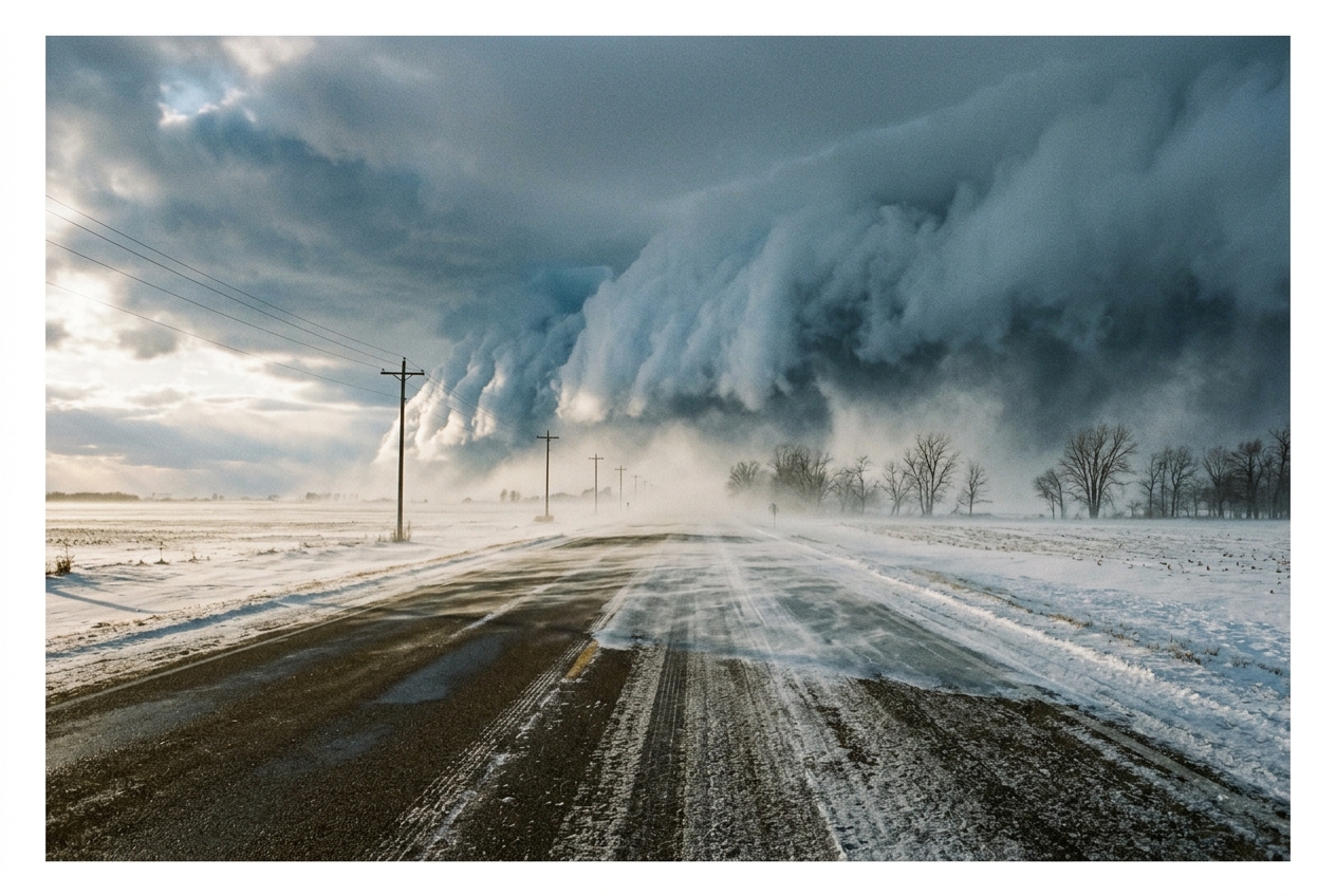
The early afternoon along the interstate corridor begins under an unassuming, slate-grey sky. The air feels deceptively calm, hovering just around freezing at $+1\text{ }^\circ\text{C}$, though a subtle, prickling dryness on the skin hints at the continental interior air mass lurking hundreds of miles to the north-west. You can smell the sharp, metallic tang of ozone and chilled mineral dust suspended in the light southerly breeze. High above, the sun is a dull alabaster disc filtered through a thin veil of altostratus, casting long, diffuse shadows across the damp, salted asphalt.
Then, within seconds, the southern horizon dissolves.
A towering, charcoal-hued roll cloud—an arcus of terrifying proportions—rushes across the open fields at motorway speed. The air pressure drops with a distinct pop in the ears, immediately followed by a violent barometric rebound as the leading gust front slams into the landscape. The southerly breeze instantly veers ninety degrees, screaming out of the north-west at fifty knots. Ambient light is extinguished, plunged into a churning, milky twilight. The temperature plummets by ten degrees Celsius in under three minutes.
Rain does not fall; instead, a horizontal barrage of razor-sharp stellar dendrites obliterates optical visibility to less than thirty metres. On the highway, the thin film of moisture on the road surface undergoes a instantaneous phase transition into a continuous, mirror-like sheet of transparent glaze. Drivers have neither the friction to brake nor the visual reference to steer. In under sixty seconds, a benign winter commute has mutated into an extreme mesoscale trap.
2. What's Actually Happening — Plain English First
To understand why a snow squall is so profoundly different from a standard winter storm, one must contrast the expansive architecture of a synoptic blizzard with the concentrated fury of mesoscale convection. A classical blizzard is an atmospheric heavyweight: a vast cyclonic system spanning thousands of kilometres, governed by slow, continuous ascent along gentle frontal surfaces over twelve to thirty-six hours according to the American Meteorological Society. A snow squall, by contrast, is a winter thunderstorm stripped of liquid rain—a hyper-localized atmospheric hammer that expends its kinetic energy in a tight thirty-to-sixty-minute burst.
Think of the atmosphere as a layered cake, where each layer possesses a distinct density and temperature profile. In a stable winter environment, cold, dense air sits quietly at the surface beneath warmer air aloft, acting like a heavy blanket that suppresses vertical motion. In a snow squall environment, however, the meteorological cake is inverted near the ground. Solar insolation through broken clouds or strong low-level warm advection warms the immediate surface layer, while an intensely cold, dry arctic air mass charges in aloft.
When the temperature drops exceptionally fast with height—what meteorologists call a steep lapse rate ($\Gamma \ge 8\text{--}9\text{ }^\circ\text{C/km}$)—the lowest two kilometres of the atmosphere become dynamically buoyant. Even tiny pockets of rising air become warmer and less dense than the surrounding deep freeze, accelerating upward like an underwater cork released from the seabed. This generates shallow Convective Available Potential Energy (CAPE), typically between $50\text{ and }150\text{ J/kg}$. While modest compared to summer supercell values, this energy is packed entirely within a shallow, sub-two-kilometre boundary layer.
This explosive updraft channels low-level moisture directly into the atmospheric "sweet spot" for snowflake generation: the Dendritic Growth Zone (DGZ), situated precisely between $-12\text{ }^\circ\text{C}\text{ and }-18\text{ }^\circ\text{C}$. Within this thermal corridor, the difference between the saturation vapor pressure over liquid water and that over ice reaches its thermodynamic maximum, a phenomenon known as the Wegener-Bergeron-Findeisen process. Water vapor sublimates directly onto ice nuclei at maximum velocity, assembling delicate, six-branched stellar dendrites. Because convective updrafts continuously resupply supercooled moisture, the crystal production rate is colossal. These wide, branching crystals possess enormous cross-sectional surface areas relative to their mass, scattering ambient photons with extreme efficiency and causing the immediate optical extinction known as a whiteout.
Simultaneously, the surface below experiences a flash freeze. Under normal conditions, road pavement acts as a massive thermal heat sink, retaining ground warmth long after air temperatures dip below freezing. However, when the squall's leading edge arrives, the combination of gale-force winds and a $10\text{--}15\text{ }^\circ\text{C}$ air temperature collapse strips heat from the pavement via forced convective cooling. The latent heat of fusion within the wet road film is rapidly overwhelmed, freezing liquid meltwater into a seamless sheet of black ice before mechanical dissipation or tire friction can displace it.
3. The Science (For Those Who Want to Go Deeper)
To mathematically forecast and diagnose the onset of severe arctic frontal convection, dynamical meteorology relies on two foundational hydrodynamic processes: kinematic frontogenesis and ageostrophic isallobaric acceleration.
A. Kinematic Frontogenesis & Deformation
Frontogenesis is the rate at which horizontal gradients of potential temperature ($\theta$) intensify over time. When an arctic air mass surges equatorward, the ambient horizontal wind field stretches and shears the thermal boundary, focusing the temperature contrast into a razor-thin zone just a few kilometres wide.
According to the classical formulation established by Sverre Petterssen and documented by the World Meteorological Organization, two-dimensional kinematic frontogenesis in the horizontal plane is defined as the Lagrangian time rate of change of the magnitude of the potential temperature gradient:
$$\mathcal{F} = \frac{d}{dt} |\nabla_h \theta| = \frac{1}{2} |\nabla_h \theta| \left( D \cos 2\alpha - \delta \right)$$
Where: * $|\nabla_h \theta| = \sqrt{\left(\frac{\partial \theta}{\partial x}\right)^2 + \left(\frac{\partial \theta}{\partial y}\right)^2}$ is the magnitude of the horizontal potential temperature gradient ($\text{K}\cdot\text{m}^{-1}$). * $D = \sqrt{E^2 + F^2}$ is the total kinematic horizontal deformation rate ($\text{s}^{-1}$), composed of stretching deformation $E = \frac{\partial u}{\partial x} - \frac{\partial v}{\partial y}$ and shearing deformation $F = \frac{\partial v}{\partial x} + \frac{\partial u}{\partial y}$. * $\alpha$ is the angle between the potential temperature gradient vector $\nabla_h \theta$ and the axis of maximum contraction of the deformation field. * $\delta = \nabla_h \cdot \mathbf{v} = \frac{\partial u}{\partial x} + \frac{\partial v}{\partial y}$ is the horizontal kinematic divergence ($\text{s}^{-1}$); thus, $-\delta$ represents horizontal convergence.
Worked Example: Frontogenetical Forcing Across a Surging Arctic Boundary
Consider an active cold front advancing over the Great Plains. Synoptic weather stations measure an initial horizontal potential temperature gradient of $8\text{ K}$ over a distance of $80\text{ km}$ ($|\nabla_h \theta| = 1.0 \times 10^{-4}\text{ K}\cdot\text{m}^{-1}$).
Mesoscale wind analysis yields: 1. Stretching deformation $E = 1.6 \times 10^{-4}\text{ s}^{-1}$ and shearing deformation $F = 1.2 \times 10^{-4}\text{ s}^{-1}$, yielding a total deformation $D = \sqrt{(1.6^2 + 1.2^2)} \times 10^{-4} = 2.0 \times 10^{-4}\text{ s}^{-1}$. 2. The axis of contraction is aligned directly parallel to the temperature gradient, such that $\alpha = 0^\circ$, making $\cos(2\alpha) = 1.0$. 3. Strong low-level kinematic convergence along the front produces a horizontal divergence value of $\delta = -1.0 \times 10^{-4}\text{ s}^{-1}$ (hence convergence $-\delta = +1.0 \times 10^{-4}\text{ s}^{-1}$).
We compute the frontogenesis function $\mathcal{F}$:
$$\mathcal{F} = \frac{1}{2} \left( 1.0 \times 10^{-4} \right) \left[ \left( 2.0 \times 10^{-4} \times 1.0 \right) - \left( -1.0 \times 10^{-4} \right) \right]$$
$$\mathcal{F} = \frac{1}{2} \left( 1.0 \times 10^{-4} \right) \left[ 2.0 \times 10^{-4} + 1.0 \times 10^{-4} \right]$$
$$\mathcal{F} = \frac{1}{2} \left( 1.0 \times 10^{-4} \right) \left( 3.0 \times 10^{-4} \right) = 1.5 \times 10^{-8}\text{ K}\cdot\text{m}^{-1}\cdot\text{s}^{-1}$$
To grasp this magnitude, convert the metric to operational forecasting units ($\text{K}\cdot(100\text{ km})^{-1}\cdot(3\text{ hr})^{-1}$):
$$\mathcal{F} = 1.5 \times 10^{-8}\text{ K}\cdot\text{m}^{-1}\cdot\text{s}^{-1} \times (10^5\text{ m}) \times (10,800\text{ s}) = 16.2\text{ K}\cdot(100\text{ km})^{-1}\cdot(3\text{ hr})^{-1}$$
B. The Isallobaric Wind Surge & Downward Momentum Transport
As the wedge of dense arctic air displaces the lighter pre-frontal air mass, surface barometric pressure rises dramatically immediately behind the gust front ($\partial p / \partial t > +3\text{ to }+6\text{ hPa / 3 hr}$). This intense spatial gradient of pressure tendency drives a powerful ageostrophic wind component known as the isallobaric wind ($\mathbf{v}_{ia}$), as detailed by the Met Office.
Derived from the Navier-Stokes equations under the quasi-geostrophic approximation on an $f$-plane, the isallobaric wind accelerates perpendicular to isallobars, blowing directly down the pressure-rise gradient into the squall line:
$$\mathbf{v}_{ia} = -\frac{1}{\rho f^2} \nabla_h \left( \frac{\partial p}{\partial t} \right)$$
Where: * $\rho$ is the mean atmospheric boundary layer air density ($\approx 1.25\text{ kg}\cdot\text{m}^{-3}$ in cold winter air). * $f = 2\Omega \sin\phi$ is the Coriolis parameter ($f \approx 1.0 \times 10^{-4}\text{ s}^{-1}$ at mid-latitudes $\phi \approx 43^\circ\text{N}$). * $\nabla_h \left( \frac{\partial p}{\partial t} \right)$ is the horizontal spatial gradient of the local time rate of change of pressure ($\text{Pa}\cdot\text{m}^{-1}\cdot\text{s}^{-1}$).
Worked Example: Calculating the Isallobaric Gale
Suppose a meso- $\beta$ network of barometers detects a sharp pressure surge. Behind the front, pressure rises at $+4.5\text{ hPa}$ in $3\text{ hours}$, while ahead of the front, pressure falls at $-1.5\text{ hPa}$ in $3\text{ hours}$. This creates a net tendency differential of $\Delta (\partial p / \partial t) = 6.0\text{ hPa / 3 hr}$ across a cross-frontal transition distance of $\Delta x = 120\text{ km} = 1.2 \times 10^5\text{ m}$.
Convert the isallobaric tendency differential to SI units:
$$\Delta\left(\frac{\partial p}{\partial t}\right) = \frac{600\text{ Pa}}{10,800\text{ s}} \approx 0.0556\text{ Pa}\cdot\text{s}^{-1}$$
Compute the horizontal gradient magnitude:
$$\left| \nabla_h \left(\frac{\partial p}{\partial t}\right) \right| = \frac{0.0556\text{ Pa}\cdot\text{s}^{-1}}{1.2 \times 10^5\text{ m}} \approx 4.63 \times 10^{-7}\text{ Pa}\cdot\text{m}^{-1}\cdot\text{s}^{-1} = 4.63 \times 10^{-7}\text{ N}\cdot\text{m}^{-3}\cdot\text{s}^{-1}$$
Now, evaluate the isallobaric ageostrophic wind speed:
$$|\mathbf{v}_{ia}| = \frac{4.63 \times 10^{-7}\text{ N}\cdot\text{m}^{-3}\cdot\text{s}^{-1}}{\left(1.25\text{ kg}\cdot\text{m}^{-3}\right) \times \left(1.0 \times 10^{-4}\text{ s}^{-1}\right)^2} = \frac{4.63 \times 10^{-7}}{1.25 \times 10^{-8}} = 37.04\text{ m}\cdot\text{s}^{-1}$$
$$|\mathbf{v}_{ia}| \approx 133.3\text{ km}\cdot\text{h}^{-1}\text{ (or } 82.8\text{ mph)}$$
Coupled with convective downward momentum transport—where vigorous downdrafts intercept the $850\text{ hPa}$ Low-Level Jet (LLJ) and drag high-momentum air directly to the ground—the isallobaric vector produces the signature non-gradient wind burst that routinely rolls articulated lorries and uproots infrastructure during squall passage.
C. The Thermodynamic Surface Energy Balance and Flash Freeze Kinetics
The instant freezing of wet highway surfaces is governed by the surface energy budget equation:
$$Q_{\text{net}} = R_n - H - LE - G$$
Where: * $R_n$ is net radiation (negative during overcast, sun-obscured winter squalls). * $H = \rho c_p C_H U (T_s - T_a)$ is the turbulent sensible heat flux. * $LE = \rho L_v C_E U (q_s - q_a)$ is the latent heat flux from evaporation/sublimation. * $G = -k \frac{\partial T}{\partial z}\Big|_{\text{surface}}$ is the conductive heat flux from the sub-pavement ground.
When the squall hits, the wind speed $U$ spikes from $3\text{ m/s to }25\text{ m/s}$, while ambient air temperature $T_a$ drops $15\text{ K}$ below the pavement temperature $T_s$. The turbulent sensible heat extraction term $H$ spikes by a factor of 20 to 30. Ground thermal conductivity $k$ through asphalt or concrete cannot supply heat upward rapidly enough to counter this atmospheric cooling. The residual meltwater film rapidly reaches the nucleation threshold ($0\text{ }^\circ\text{C}$), expels its latent heat of fusion ($L_f = 3.34 \times 10^5\text{ J/kg}$), and vitrifies into a frictionless sheet of glaze ice within four to eight minutes of frontal arrival.
4. Practical Outdoor Guidance
Operational meteorologists at the National Oceanic and Atmospheric Administration (NOAA) and the National Weather Service monitor high-resolution radar and numerical mesoscale models for the Snow Squall Parameter (SNSQ). This composite dimensionless index quantifies squall potential:
$$\text{SNSQ} = \left[ \frac{\text{CAPE}{0\text{-}2\text{km}}}{100\text{ J/kg}} \right] \times \left[ \frac{\text{RH}{0\text{-}2\text{km}}}{70\%} \right] \times \left[ \frac{|\Delta\mathbf{v}_{0\text{-}2\text{km}}|}{15\text{ m/s}} \right] \times \left[ \frac{\mathcal{F}}{10\text{ K}/(100\text{ km}\cdot 3\text{ hr})} \right]$$
When $\text{SNSQ} \ge 1.0$, all necessary ingredients for severe frontal convection synchronize. For the outdoor professional, mariner, mountaineer, or motorist, recognizing these dynamics in real time requires active field observation.
Visual and Sensory Indicators in the Field
- The Visual Horizon: Scan the upwind horizon (typically west or north-west). Look for an organized, leaden-grey shelf cloud (arcus) that appears low, jagged, and laterally continuous. If the base of the cloud is churning and trailing white virga curtains that touch the ground, the squall is in the active convective phase.
- Barometric and Thermal Signatures: Portable microbarographs (including smartphone pressure sensors) will show an abrupt inflection: a sharp, downward pressure notch followed instantly by a steep, vertical spike. If your thermometer drops from $+2\text{ }^\circ\text{C}$ to $-5\text{ }^\circ\text{C}$ while the wind backs and veers violently, frontal passage is occurring.
- Acoustic and Olfactory Shifts: Prior to squall impact, high-frequency turbulence produces a characteristic low-frequency rumble as gale-force gusts pass through treelines and structures. The smell transitions from damp road dust to the distinct, crisp purity of deep arctic air.
Rules of Action for the Outdoors
- For Motorists: Treat an active Snow Squall Warning with the same urgency as a Tornado Warning. If caught on an open highway, do not brake abruptly. Reduce speed gradually, pull entirely off the travel lanes into a designated parking area or wide shoulder, illuminate four-way hazard flashers, and keep your seatbelt fastened. Do not exit the vehicle; multiple-vehicle chain-reaction pileups occur because following drivers cannot see stationary vehicles through the whiteout.
- For Mountaineers and Hikers: The arrival of an arctic squall on exposed ridgelines elevates wind-chill hypothermia risk from moderate to immediately fatal. Drop off exposed ridgelines immediately upon sighting the western arcus cloud. Seek leeward topographic shelter before the temperature plunge and gale-force isallobaric surge destroy your ability to deploy emergency bivi shelters.
- For Coastal Sailors and Mariners: Prepare for instant, severe wind shifts accompanied by violent spray and blinding snow. Secure loose gear on deck, reef sails well in advance of the shelf cloud, and switch to radar-assisted navigation as visual references and harbor markers will vanish completely within seconds.
5. Today's Meteorological Rule of Thumb
When arctic air collides with low-level moisture and steep lapse rates, winter abandons its steady, quiet pace and adopts the violent, fast-moving dynamics of severe convection. Understanding the physics behind this transition is the difference between being blindsided by a lethal whiteout and anticipating the atmosphere's most dramatic cold-season phenomenon.