Optical Turbulence & Scintillation Dynamics: How Boundary Layer Heat Fluxes and Refractive Index Variations Forge Twinkling Stars and Horizon Shimmer
1. Opening Scene: The Shivering Horizon
Step out onto an exposed grassy ridge an hour after autumnal twilight. The ground beneath your boots is radiating the day’s warmth into the clear black void above, shedding thermal energy via longwave infrared emission. As the surface cools, a chilled, dense skin of air collects in the depressions of the turf, sliding silently downhill as a faint katabatic drainage breeze. If you kneel and touch the grass, condensation is already forming—the sharp, earthy fragrance of damp loam and fallen leaves fills the air, mingling with the crisp metallic bite of rapidly dropping ambient temperatures.
       Incoming Starlight Wavefront (Planar)
       ------------------------------------
       ||||||||||||||||||||||||||||||||||||
                  \      /
     ~ ~ ~ ~ ~ ~ ~ \ ~ ~/ ~ ~ ~ ~ ~ ~ ~ ~ ~  Warm Eddy (Lower n, diverging)
                    \  /
                     \/
     ~ ~ ~ ~ ~ ~ ~ ~ /\ ~ ~ ~ ~ ~ ~ ~ ~ ~ ~  Cold Eddy (Higher n, converging)
                    /  \
                   /    \
                 [ Observer Eye / Pupil ]
             Intensity Focuses & Blinks Rapidly
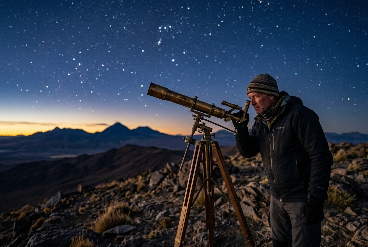
Look toward the eastern horizon. Low in the haze, Sirius—the brightest stellar beacon of the night—is engaged in a frantic, almost violent performance. It does not merely fluctuate in brightness; it shivers, jumps, and flashes with prismatic intensity, darting rapidly from sapphire blue to emerald green and ruby red in fractions of a second. Yet, cast your gaze forty degrees higher toward the southern meridian, where Jupiter commands the sky. The giant planet rests in serene, majestic equilibrium. Its creamy amber light does not flicker, tremble, or shift hue; it glows with the steady, calm luminance of a distant lantern.
Lower your gaze once more toward the valley floor below, where a dual carriageway stretches into the distance. Even under the chill of night, the residual heat rising from the dark asphalt turns the taillights of distant vehicles into writhing, liquid ribbons of red. Though the air across the landscape appears immaculately transparent to the naked eye, you are gazing through a turbulent, churning fluid whose optical properties are fractured into millions of fleeting, invisible lenses.
2. What's Actually Happening — Plain English First
To understand why the sky behaves like a kaleidoscope, we must abandon the intuitive notion that air is a uniform, static void. Instead, think of the atmosphere as a vast, turbulent river of air composed of countless interlocking transparent parcels—known to meteorologists and fluid dynamicists as turbulent eddies.
The Atmospheric Layer Cake and the Pool of Glass
Think of the atmosphere as a colossal, layered cake that has been violently stirred. Each parcel of air in this stirred mixture possesses a slightly different temperature and density from its immediate neighbours. When light passes through empty space, it travels at the unimpeded speed of light, $c$. However, as light enters the Earth's gaseous envelope, the electric fields of passing electromagnetic waves interact with the electron clouds of nitrogen and oxygen molecules, slowing the light down.
The degree to which light slows down is measured by the medium’s refractive index. Cold air is dense: its molecules are packed tightly together, forcing light to interact with more matter, which slows the wavefront and bends it inward. Warm air is rarefied and less dense: light travels faster through it, bending outward.
  PLANETARY EXTENDED DISK vs. STELLAR POINT SOURCE

   Stellar Wavefront              Planetary Wavefront
    (Single Ray Bundle)           (Multiple Uncorrelated Bundles)
          |   |                         \   |   /
     +----+---+----+               +----+---+----+
     | Turbulent   |               | Turbulent   |
     | Air Eddy    |               | Air Eddies  |
     +----+---+----+               +----+---+----+
          |   |                      \     |     /
          |   |                       \    |    /
       [ Pupil ]                         [ Pupil ]
   (Complete Blink / Fade)        (Averaged Out Constant Flux)
When you look at the bottom of a sunlit swimming pool, you see bright, dancing bands of light crisscrossing the tiles. The undulating surface ripples act as moving convex and concave lenses, focusing sunlight into bright lines and dispersing it away from the dark regions. The atmosphere does the exact same thing to starlight. As thermal plumes rise from the earth and mix with chilled sinking air, the atmosphere becomes a dynamic matrix of ephemeral optical lenses drifting across your line of sight.
The Point Source versus the Disk: Why Planets Do Not Blink
Why, then, does Sirius twinkle with incandescent fury while Jupiter remains rock-steady? The secret lies in the optical geometry of angular size:
- Stars are Optical Point Sources: Even through the most powerful ground-based research telescopes, a star is so unfathomably far away that its physical diameter subtends an angular width of less than a thousandth of an arcsecond (a sub-milliarcsecond). To an observer on Earth, starlight arrives as an infinitely narrow, coherent beam of light—a single pencil ray. When an atmospheric eddy measuring a few centimetres across drifts through this ray, the entire light bundle is deflected, focused, or defocused simultaneously. The light entering your pupil can be entirely concentrated (a blinding spike in brightness) or bent away from your eye altogether (a momentary blackout).
- Planets are Extended Disks: Although Jupiter appears as a single point of light to the unaided eye, it actually subtends an angular diameter of roughly 40 to 50 arcseconds—tens of thousands of times wider than a star. A planet is not a single point source; it is an array of millions of adjacent, independent light-emitting points. As light from the northern limb of Jupiter passes through one warm, diverging eddy, light from the southern limb simultaneously passes through an adjacent cold, converging eddy. At your eye's pupil, the random brightenings and dimmings from thousands of separate path trajectories average out. The net flux remains constant, producing a calm, unblinking radiance.
3. The Science (For Those Who Want to Go Deeper)
To move from qualitative observation to predictive meteorology, we must formalize how thermodynamics, turbulence spectra, and electrodynamics govern the propagation of light through the planetary boundary layer and free troposphere.
Refractive Index Coupling: The Gladstone-Dale and Edlén Formulations
The optical behavior of air begins with its physical density, $\rho$. The classical Gladstone-Dale relation states that the refractive index $n$ of a gas is linearly proportional to its mass density:
$$n - 1 = K_{\text{GD}} \cdot \rho$$
where $K_{\text{GD}}$ is the Gladstone-Dale constant (approximately $0.226 \times 10^{-3}\text{ m}^3/\text{kg}$ for dry air at visible wavelengths). Utilizing the ideal gas equation of state, $\rho = \frac{P}{R_{\text{spec}} T}$, where $P$ is absolute barometric pressure, $T$ is absolute temperature in Kelvin, and $R_{\text{spec}} \approx 287.05\text{ J}/(\text{kg}\cdot\text{K})$ is the specific gas constant for dry air, we obtain the standard meteorological refractivity formula (adapted from the Edlén equation):
$$n(T, P) - 1 \approx 79 \times 10^{-6} \cdot \frac{P}{T}$$
Here, $P$ is expressed in hectopascals ($\text{hPa}$) and $T$ in Kelvin ($\text{K}$).
In the open atmosphere, high-frequency pressure perturbations equilibrate rapidly at the local speed of sound ($c_s \approx 340\text{ m/s}$). Microscale acoustic waves disperse pressure anomalies across metres in milliseconds. Consequently, microscale turbulent fluctuations are virtually isobaric ($\delta P \approx 0$). Taking the partial derivative of $n$ with respect to temperature under constant pressure yields:
$$\frac{\partial n}{\partial T} = -79 \times 10^{-6} \cdot \frac{P}{T^2}$$
$$\delta n \approx -\left(79 \times 10^{-6} \cdot \frac{P}{T^2}\right) \delta T$$
Physical Insight: A microthermal fluctuation $\delta T$ of merely $0.1\text{ K}$ at sea level ($P = 1013.25\text{ hPa}$, $T = 288.15\text{ K}$) produces a refractive index variation:
$$\delta n \approx -\left(79 \times 10^{-6} \cdot \frac{1013.25}{(288.15)^2}\right) (0.1) \approx -9.64 \times 10^{-8}$$
While an alteration in the eighth decimal place seems negligible, starlight traversing several vertical kilometres of air accumulates thousands of these phase retardations, corrupting an otherwise pristine, planar optical wavefront into an intricately crumpled, chaotic surface.
Kolmogorov Turbulence and the Refractive Index Structure Parameter ($C_n^2$)
Atmospheric kinetic energy enters the system at large macro-scales (the outer scale $L_0$, typically $10\text{ to }100\text{ metres}$), driven by solar surface heating, thermal convection, and synoptic-scale wind shear. According to Kolmogorov's cascade theory, these large buoyant plumes break down into successively smaller vortices within the inertial subrange, transferring their kinetic energy without viscous dissipation until reaching the inner scale ($l_0$, typically $1\text{ to }10\text{ millimetres}$), where molecular viscosity finally dissipates the energy into heat.
When temperature gradients are entrained in this cascade, the scalar temperature field behaves identically according to the Obukhov-Corrsin spectrum. The statistical variation of temperature between two points separated by a spatial distance vector $\mathbf{r}$ (where $l_0 \ll |\mathbf{r}| \ll L_0$) is quantified by the temperature structure function $D_T(r)$:
$$D_T(r) = \langle [T(\mathbf{x}) - T(\mathbf{x} + \mathbf{r})]^2 \rangle = C_T^2 \cdot r^{2/3}$$
where $C_T^2$ is the temperature structure constant (in units of $\text{K}^2\cdot\text{m}^{-2/3}$).
Coupling this statistical temperature variance directly to our refractivity gradient yields the refractive index structure function $D_n(r)$:
$$D_n(r) = \langle [n(\mathbf{x}) - n(\mathbf{x} + \mathbf{r})]^2 \rangle = C_n^2 \cdot r^{2/3}$$
where $C_n^2$ represents the quintessential optical turbulence parameter, the refractive index structure constant:
$$C_n^2 = \left(7.9 \times 10^{-5} \cdot \frac{P}{T^2}\right)^2 \cdot C_T^2 \quad [\text{m}^{-2/3}]$$
| Atmospheric Environment | Typical $C_n^2$ Magnitude ($\text{m}^{-2/3}$) | Optical Impact on Observers |
|---|---|---|
| Intense Boundary Layer (Sunbaked desert, hot tarmac) | $10^{-12} \text{ to } 10^{-11}$ | Severe daytime heat shimmering; distant objects liquefy. |
| Moderate Surface Layer (Breezy nocturnal prairie) | $10^{-14} \text{ to } 10^{-13}$ | Rapid naked-eye star scintillation; visible twinkling. |
| High-Altitude Observatories (Mauna Kea, Paranal) | $10^{-16} \text{ to } 10^{-15}$ | Exceptional stellar stability; planetary fine detail resolved. |
| Free Troposphere / Stratosphere (Calm upper atmosphere) | $10^{-18} \text{ to } 10^{-17}$ | Near-diffraction-limited optical propagation. |
Wave Propagation, the Scintillation Index, and Air Mass
As an unperturbed plane wave from a distant star enters the top of the atmosphere, it possesses flat, parallel surfaces of constant optical phase. Passing through inhomogeneous distributions of $C_n^2(z)$, phase aberrations develop. Propagating further downward, these crumpled wavefronts interfere with themselves, redistributing optical energy into localized intensity spikes and nulls.
Under the Rytov perturbation approximation for weak optical turbulence, the variance of normalized optical intensity fluctuations—termed the scintillation index $\sigma_I^2$—is derived analytically:
$$\sigma_I^2 = \frac{\langle I^2 \rangle - \langle I \rangle^2}{\langle I \rangle^2} = 1.23 \cdot C_n^2 \cdot k^{7/6} \cdot L^{11/6}$$
Where: * $k = \frac{2\pi}{\lambda}$ is the optical wavenumber (for green light $\lambda = 550\text{ nm} = 5.5 \times 10^{-7}\text{ m}$, $k \approx 1.142 \times 10^7\text{ rad/m}$). * $L$ is the total optical propagation path length through the turbulent layer.
For an astronomical object observed at a zenith angle $\zeta$ (the angle between the celestial target and the local vertical), the effective atmospheric path length scales with the secant of the zenith angle:
$$L(\zeta) = L_0 \cdot \sec(\zeta) = \frac{L_0}{\cos(\zeta)}$$
Substituting this path dependence into our scintillation equation reveals the severe geometric penalty incurred near the horizon:
$$\sigma_I^2(\zeta) = 1.23 \cdot C_n^2 \cdot k^{7/6} \cdot (L_0 \sec\zeta)^{11/6} \propto (\sec\zeta)^{1.833}$$
                Zenith (zeta = 0 deg)
                     |  Air Mass = 1.0
                     |  Shortest Path (L_0)
                     |  Minimal Scintillation
                    / \
                   /   \
                  /     \
                 /       \
                /         \
  Low Horizon              Low Horizon
  (zeta = 75 deg)          (zeta = 75 deg)
  Air Mass = 3.86          Air Mass = 3.86
  Path = 3.86 * L_0        Path = 3.86 * L_0
  Severe Scintillation     Severe Scintillation
When an object is near the horizon ($\zeta = 75^\circ$, $\sec\zeta \approx 3.86$), starlight must traverse nearly four times as much turbulent air mass as an object at the zenith. Because $\sigma_I^2 \propto (\sec\zeta)^{11/6}$, the intensity variance increases by $(3.864)^{1.833} \approx 11.9\text{-fold}$. This dramatic amplification explains why stars near the horizon flash and dance like dying flares, while the same stars settle into moderate stability when climbing overhead.
The Fried Coherence Parameter ($r_0$) and Spatial Coherence
To measure the overall optical quality of the atmosphere (which astronomers refer to as astronomical seeing), David L. Fried formulated the coherence length $r_0$. The Fried parameter $r_0$ represents the spatial diameter across a telescope aperture over which the optical wavefront's root-mean-square phase distortion remains less than 1 radian:
$$r_0 = \left( 0.423 \cdot k^2 \cdot \sec(\zeta) \int_0^\infty C_n^2(z) \, dz \right)^{-3/5}$$
Notice the fundamental properties embedded in this equation: 1. Wavelength Dependence ($r_0 \propto \lambda^{6/5}$): The spatial coherence diameter is noticeably larger at longer wavelengths. Infrared light experiences significantly less phase distortion and scintillation than blue or ultraviolet light. 2. Atmospheric Seeing Limit: An optical telescope with an aperture diameter $D$ significantly larger than $r_0$ cannot achieve its theoretical diffraction-limited angular resolution ($\theta \approx 1.22 \frac{\lambda}{D}$). Instead, its resolution is clamped to the seeing disk:
$$\theta_{\text{seeing}} \approx \frac{\lambda}{r_0}$$
On an average night at sea level, $r_0$ typically measures between $5\text{ cm}$ and $10\text{ cm}$. A multi-metre research telescope looking up without adaptive optics will resolve no more spatial detail than a modest 10-centimetre amateur telescope.
       WAVEFRONT ARRIVING AT APERTURE

       Ideal Plane Wave:
       ---------------------------------  (Diffraction limit: theta = 1.22 * lambda / D)

       Turbulent Wavefront:
       ~~~\_____/~~~\________/~~~\______  (Seeing limit: theta = lambda / r_0)
       |<-- r_0 -->|
       Coherent patch
Worked Numerical Example: Sirius at Zenith vs. the Horizon
Let us model a concrete, real-world scenario to calculate exact values for $C_n^2$, $r_0$, and $\sigma_I^2$.
Scenario Parameters:
- Wavelength: $\lambda = 550\text{ nm}$ (Green visible light, $k = 1.1424 \times 10^7\text{ m}^{-1}$)
- Surface Meteorology: $P = 1013.25\text{ hPa}$, $T = 280\text{ K}$ ($6.85^\circ\text{C}$)
- Boundary Layer Microthermals: Micro-thermocouple probes measure a local temperature structure parameter $C_T^2 = 0.04\text{ K}^2\cdot\text{m}^{-2/3}$ within an active turbulent surface layer of effective thickness $L_0 = 1,500\text{ m}$.
Step 1: Calculate the Refractive Index Structure Constant ($C_n^2$)
Using our microthermal coupling equation:
$$C_n^2 = \left( 7.9 \times 10^{-5} \cdot \frac{P}{T^2} \right)^2 \cdot C_T^2$$
$$7.9 \times 10^{-5} \cdot \frac{1013.25}{(280)^2} = 7.9 \times 10^{-5} \cdot \frac{1013.25}{78,400} = 7.9 \times 10^{-5} \cdot 0.012924 \approx 1.021 \times 10^{-6}\text{ K}^{-1}$$
Squaring this term:
$$(1.021 \times 10^{-6})^2 \approx 1.042 \times 10^{-12}\text{ K}^{-2}$$
Multiplying by $C_T^2 = 0.04\text{ K}^2\cdot\text{m}^{-2/3}$:
$$C_n^2 = (1.042 \times 10^{-12}) \cdot 0.04 = 4.168 \times 10^{-14}\text{ m}^{-2/3}$$
This is a classic moderate turbulence value for a nocturnal boundary layer.
Step 2: Compute Scintillation Index ($\sigma_I^2$) at Zenith ($\zeta = 0^\circ$)
At the zenith, $\sec(0^\circ) = 1.0$, so $L = 1,500\text{ m}$.
- Compute $k^{7/6}$: $$k^{7/6} = (1.1424 \times 10^7)^{7/6} = (1.1424 \times 10^7)^{1.16667} \approx 1.625 \times 10^8\text{ m}^{-7/6}$$
- Compute $L^{11/6}$: $$L^{11/6} = (1,500)^{1.83333} \approx 657,340\text{ m}^{11/6}$$
- Evaluate the scintillation index: $$\sigma_I^2(\text{zenith}) = 1.23 \cdot C_n^2 \cdot k^{7/6} \cdot L^{11/6}$$ $$\sigma_I^2(\text{zenith}) = 1.23 \cdot (4.168 \times 10^{-14}) \cdot (1.625 \times 10^8) \cdot (657,340) \approx 0.548$$
A scintillation index of $\sigma_I^2 \approx 0.55$ corresponds to visible, moderate twinkling—well within the domain of weak Rytov perturbation theory ($\sigma_I^2 < 1.0$).
Step 3: Compute Scintillation Index ($\sigma_I^2$) for Sirius at Horizon ($\zeta = 75^\circ$)
At an elevation angle of $15^\circ$ above the horizon ($\zeta = 75^\circ$):
$$\sec(75^\circ) = \frac{1}{\cos(75^\circ)} \approx 3.8637$$
The effective slant optical path through the turbulent layer becomes:
$$L_{\text{slant}} = 1,500 \cdot 3.8637 \approx 5,795.5\text{ m}$$
Evaluating $L_{\text{slant}}^{11/6}$:
$$L_{\text{slant}}^{11/6} = (5,795.5)^{1.83333} \approx 7,819,000\text{ m}^{11/6}$$
Substituting into the scintillation index formula:
$$\sigma_I^2(75^\circ) = 1.23 \cdot (4.168 \times 10^{-14}) \cdot (1.625 \times 10^8) \cdot (7,819,000) \approx 6.51$$
Physical Interpretation: A scintillation index of $\sigma_I^2 = 6.51$ drastically exceeds unity, placing this light path deep into the strong saturation regime. Starlight is no longer merely experiencing mild phase wobbles; the light field has fractured into multiple chaotic speckle interference patterns. Extreme destructive interference causes the star to completely vanish for milliseconds at a time, followed by extreme constructive caustic spikes.
Furthermore, because the refractive index $n(\lambda)$ varies slightly with wavelength (dispersion), red, green, and blue wavelengths are refracted along physically separate geometric paths through different turbulent cells. The red, green, and blue foci strike the observer’s retina at alternating intervals, producing the brilliant chromatic flashing characteristic of low-altitude stars.
Step 4: Compute the Fried Parameter ($r_0$)
Assuming our turbulent layer of $C_n^2 = 4.168 \times 10^{-14}\text{ m}^{-2/3}$ extends over $L = 1,500\text{ m}$, the integrated turbulence profile is:
$$\int_0^\infty C_n^2(z) \, dz = C_n^2 \cdot L_0 = (4.168 \times 10^{-14}) \cdot 1,500 = 6.252 \times 10^{-11}\text{ m}^{1/3}$$
Now evaluate $r_0$ at the zenith ($\zeta = 0^\circ$):
$$r_0 = \left( 0.423 \cdot k^2 \cdot \int C_n^2(z) \, dz \right)^{-3/5}$$
- Compute $k^2$: $$k^2 = (1.1424 \times 10^7)^2 \approx 1.305 \times 10^{14}\text{ m}^{-2}$$
- Compute the bracketed product: $$0.423 \cdot (1.305 \times 10^{14}) \cdot (6.252 \times 10^{-11}) \approx 3,451.2\text{ m}^{-5/3}$$
- Take the $-3/5$ power: $$r_0 = (3,451.2)^{-0.6} \approx 0.0742\text{ m} = 7.42\text{ cm}$$
The atmosphere on this evening limits diffraction-limited optical coherence to an aperture of just $7.42\text{ cm}$. The corresponding astronomical seeing disk is:
$$\theta_{\text{seeing}} \approx \frac{\lambda}{r_0} = \frac{5.5 \times 10^{-7}\text{ m}}{0.0742\text{ m}} \approx 7.41 \times 10^{-6}\text{ rad} \approx 1.53\text{ arcseconds}$$
4. Practical Outdoor Guidance
Armed with an understanding of microthermal turbulence and optical wave propagation, an outdoor observer, weather watcher, or astrophotographer can diagnose the stability of the atmosphere using simple visual observations and basic meteorological instruments.
       SUMMARY OBSERVATIONAL MATRIX

  NIGHT SKY PHENOMENON             UPPER AIR STATE           BOUNDARY LAYER
  -------------------------------------------------------------------------
  Bright stars blinking violently  Strong jet stream shear   Active convection /
  at zenith (Pickering 1-3)        (200-300 hPa turbulence)  thermal plumes

  Stars steady at zenith;          Laminar zonal flow;       Ground inversion /
  planets sharp (Pickering 8-10)   thermal stability aloft   calm cold drainage
1. What to Look For in the Sky
- The Pickering Seeing Scale: Amateur astronomers and meteorologists rate optical seeing on the Pickering scale, from 1 (a star's image is a boiling, unrecognizable blob) to 10 (a perfectly steady central Airy disk surrounded by unbroken concentric diffraction rings).
- Naked-Eye Scintillation Frequency: Observe stars located near the zenith ($>60^\circ$ altitude):
- If overhead stars twinkle visibly to your unaided eye, high-altitude optical turbulence is intense ($C_n^2$ aloft is elevated). Atmospheric seeing is poor ($r_0 < 5\text{ cm}$).
- If overhead stars shine with dead, unblinking stillness and only stars below $20^\circ$ altitude flicker, the upper troposphere is quiescent and laminar. Atmospheric seeing is superb ($r_0 > 15\text{ cm}$).
- Chromatic Flashing: Look at bright stars (such as Sirius, Vega, or Capella) within $30^\circ$ of the horizon. Rapid, prismatic colour-switching indicates extreme differential dispersion coupled with strong-regime scintillation ($\sigma_I^2 > 5$), revealing intense thermal mixing in the lower $2\text{ km}$ boundary layer.
2. Instrument Readings to Monitor
- Barometric Trends (NOAA Data Access): Rapidly falling barometric pressure ($>2\text{ hPa/hr}$) indicates the approach of an upper-level trough, cold front, or baroclinic wave. Frontal zones generate violent vertical wind shear, driving intense microthermal mixing and collapsing $r_0$ to poor values. Conversely, broad, slow-moving barometric highs generally suppress vertical turbulence.
- Surface Thermometers and Dew Point Inversions: On clear, calm nights under high pressure, radiative ground cooling produces a temperature inversion (where ground temperature is cooler than the air 10 metres above). Once this inversion sets in and surface winds fall below $2\text{ m/s}$, vertical convective turbulence ceases, and boundary layer $C_n^2$ plummets.
- Upper-Level Wind Shear (Jet Stream Analysis via Met Office & WMO): Check synoptic maps for the position of the 200–300 hPa jet stream. If a 100-knot jet core sits directly overhead, mechanical shear across the tropopause creates intense layers of optical turbulence, ruining telescopic seeing even if the ground air is completely calm.
5. Today's Meteorological Rule of Thumb
The Observer’s Law of Scintillation: "When overhead stars flash and dance like frantic fireflies, violent wind shear churns the upper atmosphere; when planets burn like steady beacons and stars hold still at the zenith, a calm and stable atmosphere crowns the night."
Further Reading & Meteorological Resources
- Understand optical turbulence tracking through the NOAA Physical Sciences Laboratory.
- Explore atmospheric optical phenomena with the UK Met Office Learning Portal.
- Review international standards for meteorological observing via the World Meteorological Organization.
- Study high-resolution wave propagation theory via Astronomical Seeing on Wikipedia and Atmospheric Scintillation.