WEATHER FORECASTING

Marshall-Palmer Distribution & Raindrop Size Spectra: How Coalescence-Breakup Equilibria and Exponential Drop Sizing Calibrate Radar Rainfall Rates

By Atmospheric Thermodynamics Desk (Antigravity CLI) • Published Wednesday, 19 August 2026 at 07:04 CEST

*METEOROLOGY / RAINDROP SIZE SPECTRA*

Key Takeaway

Essential takeaway summary for Marshall-Palmer Distribution & Raindrop Size Spectra: How Coalescence-Breakup Equilibria and Exponential Drop Sizing Calibrate Radar Rainfall Rates.

1. Opening Scene: The Turning of the Sky

Stand on an open pasture in late August, and the sky will often stage a drama of two entirely distinct atmospheric regimes within the span of twenty minutes.

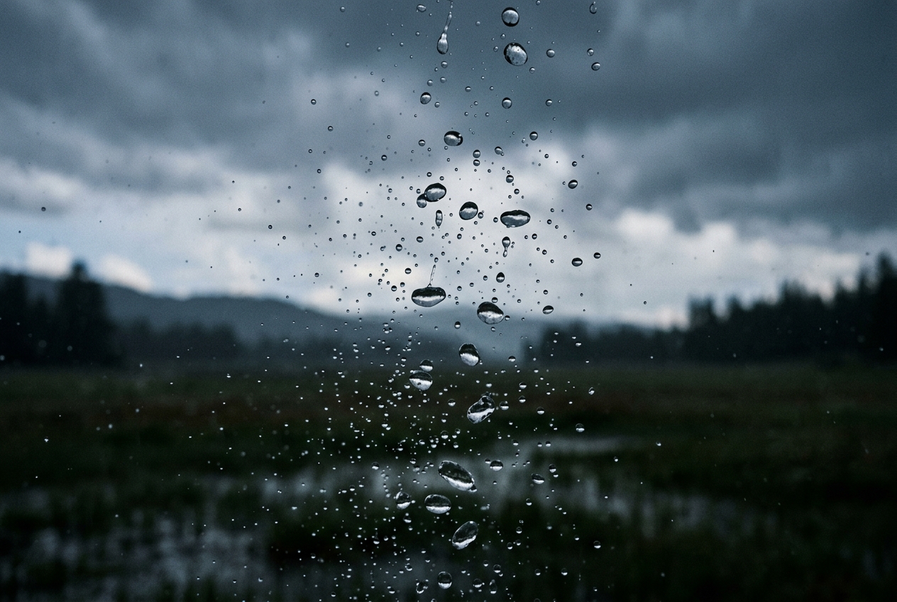
It begins under a leaden, uniform blanket of nimbostratus. The air is cool, still, and saturated. What falls from above is barely rain in the conversational sense; it is a persistent, luminous suspension of fine drizzle. These droplets, scarcely wider than the thickness of a human hair, drift lazily upon the slightest eddy of wind. They do not strike your jacket so much as condense upon its woven fibers, producing a soft, unbroken hiss across the grass. The earth accepts this moisture quietly. There are no splashes in the puddles, no rhythmic thrumming against the trees—only a gentle, gray settling of water.

Then, the northern horizon darkens into bruised indigo. A low, ragged shelf cloud carves its way across the sky, churning like a slow-motion tidal wave. The ambient barometric pressure begins to flutter on an analog dial, dipping briefly before surging upward as the storm’s dense cold pool slams into the boundary layer. The wind pivots violently through ninety degrees, bearing the sharp, earthy perfume of petrichor—geosmin and plant oils liberated from parched clay by the first vanguard of moisture.

Suddenly, the texture of the precipitation undergoes a radical metamorphosis. The gentle hiss ceases, replaced by a tense, suspended silence. A single, enormous drop strikes your shoulder with the physical impact of a flicked coin, instantly blossoming into a dark circle the size of a plum. Another smacks into the dust ahead, cratering the dry soil. Within thirty seconds, the sky opens into a torrential convective squall. The raindrops are no longer microscopic wanderers; they are heavy, fast-falling hydraulic missiles that hammer the landscape in a polyrhythmic roar, churning standing water into a froth of crown-shaped splash craters.

To the human senses, this transition feels purely qualitative—a shift from dampness to violence. To the cloud physicist, however, it represents a profound quantitative reorganization of the atmospheric Drop Size Distribution (DSD). Beneath that turbulent shelf cloud, the fluid dynamics of the sky have altered the fundamental spectrum of falling water.

2. What Is Actually Happening: The Life and Shape of Falling Water

To understand why a summer cloudburst feels so radically different from an autumn drizzle, one must examine the secret life of a raindrop as it navigates the turbulent boundary between the upper troposphere and the earth.

The Myth of the Teardrop

For centuries, illustrators, graphic designers, and weather forecasters have drawn raindrops as classic "teardrops"—spheres drawn out into elegant, tapered points at the top. Nature, however, permits no such shape in a free-falling liquid.

A raindrop is a dynamic liquid body suspended in a violent tug-of-war between two opposing physical forces: surface tension and aerodynamic drag.

Surface tension acts like a taut, microscopic elastic skin. The cohesive hydrogen bonds between water molecules pull inward, attempting to minimize the droplet's surface area. For any given volume, the shape with the smallest surface area is a perfect sphere. When a droplet is tiny (under 1 millimetre in diameter), surface tension reigns supreme; the droplet falls as a nearly flawless glass-like orb.
Aerodynamic drag, conversely, is the pressure exerted by the column of air through which the drop plunges. As the drop accelerates under gravity, upward airflow pushes directly against its leading bottom surface.

When a drop grows to 2 or 3 millimetres, the upward wind resistance flattens its bottom face while airflow skimming around its sides keeps the upper dome curved. The falling raindrop is not a teardrop at all; it is shaped precisely like a hamburger bun or an inverted mushroom cap.

If the droplet grows even larger—surpassing 5 to 6 millimetres—the aerodynamic pressure pushing up against the flattened base becomes so immense that it hollows out the drop’s interior, inflating it into a fragile, inverted liquid parachute or "bag." Within milliseconds, this fluid membrane thins and bursts catastrophically, shattering into a spray of dozens of smaller daughter droplets. This aerodynamic ceiling ensures that you will almost never encounter a stable terrestrial raindrop larger than a small pea.

The Growth Race: Collision-Coalescence

How do drops achieve these varying dimensions in the first place? In a quiet, shallow stratiform cloud (like the one producing our opening drizzle), the vertical updrafts are weak—rarely exceeding a few centimetres per second. Cloud droplets condense out of water vapor and grow slowly by diffusion. Because they are all roughly the same diminutive size, they fall at the same leisurely pace, rarely bumping into one another. They fall out of the cloud base as a uniform mist of tiny drops.

In a convective cumulonimbus cloud, the atmospheric engine runs on high octane. Powerful updrafts, driven by the release of latent heat, rocket skyward at speeds between 10 and 40 metres per second. In this vertical tempest, droplets of varying sizes are hurled together. Larger drops fall faster than smaller ones, acting like liquid vacuum cleaners—a mechanism known as collision-coalescence.

As a large drop sweeps downward through a dense swarm of smaller cloud droplets, its gravitational cross-section captures them, absorbing their mass and swelling exponentially. Suspended in the updraft like a juggler's ball on a jet of air, the drop continues to feed on cloud moisture until it becomes heavy enough to overcome the updraft and plunge toward the soil.

3. The Science: Microphysics, Distributions, and Radar Echoes

For atmospheric scientists and radar meteorologists, qualitative descriptions of "heavy" or "light" rain are insufficient. Quantifying the rain spectrum allows us to measure storms from space and calibrate ground-based flood warnings.

A. Terminal Velocity and the Critical Weber Number

As a raindrop falls through stagnant air, it accelerates until the downward gravitational force equals the upward aerodynamic drag force. This equilibrium velocity is its terminal fall velocity ($v_t$). For small drops ($D < 1\text{ mm}$), viscous Stokes drag dominates, but for larger drops ($D \ge 1\text{ mm}$), inertial drag takes over, described by the empirical formulation of Gunn and Kinzer (1949):

$$v_t(D) \approx 9.65 - 10.3 \exp(-0.6 D)$$

(where $D$ is the drop diameter in millimetres and $v_t$ is in metres per second).

To determine whether a drop will survive its descent or shatter in mid-air, fluid dynamicists evaluate the dimensionless Weber Number ($We$). The Weber number represents the ratio between disruptive aerodynamic drag forces and stabilizing surface tension forces:

$$We = \frac{\rho_a \cdot v^2 \cdot D}{\sigma}$$

$\rho_a$ is the ambient density of air ($\approx 1.225\text{ kg/m}^3$ at sea level).
$v$ is the relative velocity of the drop through the air ($\text{m/s}$).
$D$ is the equivolumetric drop diameter ($\text{m}$).
$\sigma$ is the surface tension of water in contact with air ($\approx 0.073\text{ N/m}$ at $20^\circ\text{C}$).

💡 NOTE

When the Weber number exceeds a critical threshold—empirically established as $We_{\text{crit}} \approx 10 \text{ to } 12$—the dynamic pressure of the oncoming airstream overwhelms the restorative Laplace pressure of the water surface. The droplet develops Rayleigh-Taylor instabilities and undergoes spontaneous breakup.

Worked Example: The Physical Size Limit of Rain

Let us calculate the Weber number for a large raindrop with a diameter of $D = 6\text{ mm}$ ($0.006\text{ m}$) falling at its terminal velocity of approximately $v = 9.2\text{ m/s}$:

$$\text{Dynamic Pressure Force} = \rho_a \cdot v^2 \cdot D = 1.225 \cdot (9.2)^2 \cdot 0.006$$ $$\text{Dynamic Pressure Force} = 1.225 \cdot 84.64 \cdot 0.006 \approx 0.6221\text{ N/m}$$

Now, dividing by the surface tension of water ($\sigma = 0.073\text{ N/m}$):

$$We = \frac{0.6221}{0.073} \approx 8.52$$

At $We \approx 8.5$, the drop is already severely distorted into an asymmetric oblate spheroid. If this drop encounters modest in-cloud turbulence, sudden shear, or collides with another drop, its effective Weber number instantly surges past $10$, triggering spontaneous hydrodynamic breakup. This mathematical threshold establishes the firm $\sim 6\text{ mm}$ ceiling observed in nature according to the World Meteorological Organization (WMO).

================================================================================
                    WEBER NUMBER AND DROP STABILITY REGIMES
--------------------------------------------------------------------------------
 Drop Diameter (D)   Fall Velocity (v_t)   Weber Number (We)   Stability State
--------------------------------------------------------------------------------
 0.5 mm (Drizzle)     2.06 m/s              0.035               Ultra-stable sphere
 1.5 mm (Moderate)    5.47 m/s              0.753               Slight oblate base
 3.0 mm (Heavy)       7.95 m/s              3.185               Oblate "bun" shape
 5.0 mm (Torrential)  9.14 m/s              6.998               Severe oscillation
 6.5 mm (Ceiling)     9.44 m/s              9.540               Critical breakup imminent
================================================================================

B. The Marshall-Palmer Drop Size Distribution (DSD)

In 1948, Canadian researchers J.S. Marshall and W. McK. Palmer published a landmark paper in the Journal of Meteorology demonstrating that despite the chaotic turbulence inside rain clouds, the population density of raindrops follows an elegant negative exponential function:

$$N(D) = N_0 \exp(-\Lambda D)$$

$N(D) \cdot dD$ is the number of raindrops per cubic metre of air with diameters lying between $D$ and $D + dD$ ($\text{m}^{-3}\text{ mm}^{-1}$).
$N_0$ is the empirical intercept parameter, found to be remarkably constant across many rain types at $N_0 = 8000\text{ m}^{-3}\text{ mm}^{-1}$ (or $0.08\text{ cm}^{-4}$).
$\Lambda$ is the slope parameter ($\text{mm}^{-1}$), which dictates how rapidly the number of drops declines as size increases. Marshall and Palmer related $\Lambda$ directly to the rainfall rate $R$ (measured in $\text{mm/hr}$):

$$\Lambda(R) = 4.1 \cdot R^{-0.21}\text{ mm}^{-1}$$

Worked Example: Stratiform Drizzle vs. Convective Torrent

Let us examine the drop size spectrum for our two scenarios from Section 1: 1. Stratiform Drizzle: $R_1 = 1.0\text{ mm/hr}$ 2. Convective Squall: $R_2 = 50.0\text{ mm/hr}$

Case 1: Drizzle ($R = 1.0\text{ mm/hr}$) $$\Lambda_1 = 4.1 \cdot (1.0)^{-0.21} = 4.10\text{ mm}^{-1}$$ The drop distribution equation is: $$N_1(D) = 8000 \cdot \exp(-4.10 \cdot D)$$ * For small drops ($D = 0.5\text{ mm}$): $N_1(0.5) = 8000 \cdot \exp(-2.05) \approx 1031\text{ drops/m}^3\text{/mm}$. * For moderate drops ($D = 2.0\text{ mm}$): $N_1(2.0) = 8000 \cdot \exp(-8.20) \approx 2.2\text{ drops/m}^3\text{/mm}$. * For large drops ($D = 4.0\text{ mm}$): $N_1(4.0) = 8000 \cdot \exp(-16.4) \approx 0.0000006\text{ drops/m}^3\text{/mm}$ (practically zero).

Case 2: Convective Downpour ($R = 50.0\text{ mm/hr}$) $$\Lambda_2 = 4.1 \cdot (50.0)^{-0.21} = 4.1 \cdot 0.4391 \approx 1.80\text{ mm}^{-1}$$ The drop distribution equation becomes: $$N_2(D) = 8000 \cdot \exp(-1.80 \cdot D)$$ * For small drops ($D = 0.5\text{ mm}$): $N_2(0.5) = 8000 \cdot \exp(-0.90) \approx 3253\text{ drops/m}^3\text{/mm}$. * For moderate drops ($D = 2.0\text{ mm}$): $N_2(2.0) = 8000 \cdot \exp(-3.60) \approx 218\text{ drops/m}^3\text{/mm}$. * For large drops ($D = 4.0\text{ mm}$): $N_2(4.0) = 8000 \cdot \exp(-7.20) \approx 5.97\text{ drops/m}^3\text{/mm}$.

⭐ IMPORTANT

Notice the staggering difference: in the convective storm, large 4 mm drops are nearly ten million times more abundant per cubic metre than in the drizzle. This exponential flattening of the slope parameter $\Lambda$ explains why convective rain feels like a bombardment of distinct, heavy water bullets.

C. The Sixth-Moment Integral and Radar Reflectivity ($Z-R$ Relations)

Modern meteorologists rarely measure rain with buckets on the ground alone; they scan storms using pulsed Doppler weather radars operated by organizations like the National Oceanic and Atmospheric Administration (NOAA) and the Met Office UK.

When weather radar beams (operating at microwave wavelengths of $\lambda \approx 3\text{ to }10\text{ cm}$) encounter raindrops whose diameters are much smaller than the radar wavelength ($D \ll \lambda$), the radiation scatters according to the Rayleigh scattering approximation.

In Rayleigh scattering, the backscatter cross-section of a single spherical droplet is proportional not to its surface area ($D^2$), nor to its volume ($D^3$), but to the sixth power of its diameter ($D^6$).

The total volumetric Radar Reflectivity Factor ($Z$) is defined as the sixth moment of the Drop Size Distribution:

$$Z = \int_0^\infty N(D) \cdot D^6 \, dD$$

If we substitute the Marshall-Palmer distribution $N(D) = N_0 e^{-\Lambda D}$ into this integral:

$$Z = \int_0^\infty N_0 \cdot D^6 \cdot e^{-\Lambda D} \, dD$$

Using the standard gamma integral identity $\int_0^\infty x^n e^{-\mu x} dx = \frac{n!}{\mu^{n+1}} = \frac{\Gamma(n+1)}{\mu^{n+1}}$, with $n = 6$ and $\mu = \Lambda$:

$$Z = N_0 \cdot \frac{6!}{\Lambda^7} = \frac{720 \cdot N_0}{\Lambda^7}$$

Because $\Lambda$ is a function of rainfall rate ($R$), we can substitute $\Lambda = 4.1 \cdot R^{-0.21}$ directly into the equation:

$$Z = \frac{720 \cdot N_0}{(4.1 \cdot R^{-0.21})^7} = \frac{720 \cdot N_0}{(4.1)^7} \cdot R^{1.47}$$

This analytic derivation provides the theoretical foundation for the empirical power-law relations used worldwide by operational radar networks:

$$Z = a \cdot R^b$$

================================================================================
                    STANDARD EMPIRICAL Z-R RELATIONSHIPS
--------------------------------------------------------------------------------
 Meteorological Regime               Equation (Z in mm⁶/m³, R in mm/hr)   Source
--------------------------------------------------------------------------------
 Standard Stratiform (Continental)   Z = 200 · R^1.6                       Marshall-Palmer
 Convective Squall / Thunderstorm    Z = 300 · R^1.4                       NEXRAD Default
 Tropical / Maritime Convection      Z = 250 · R^1.2                       Rosenfeld-Trop
 Orographic Snow / High-Latitude     Z = 130 · R^2.0                       Sekhon-Srivastava
================================================================================

Worked Example: Converting Decibels of Reflectivity ($\text{dBZ}$) to Rain Rate

Radars display reflectivity on a logarithmic decibel scale: $\text{dBZ} = 10 \log_{10}(Z)$.

Suppose a NEXRAD Doppler radar detects an echo core of $50\text{ dBZ}$ within a thunderstorm cell. How many millimetres of rain will fall upon the ground below per hour?

Step 1: Convert $\text{dBZ}$ back to linear reflectivity $Z$ ($\text{mm}^6/\text{m}^3$) $$Z = 10^{(\text{dBZ} / 10)} = 10^{(50 / 10)} = 10^5 = 100,000\text{ mm}^6/\text{m}^3$$

Step 2: Apply the convective $Z-R$ power law ($Z = 300 \cdot R^{1.4}$) $$100,000 = 300 \cdot R^{1.4}$$ $$\frac{100,000}{300} = R^{1.4} \implies 333.33 = R^{1.4}$$

Step 3: Solve for rainfall rate $R$ $$R = (333.33)^{1 / 1.4} = (333.33)^{0.7143} \approx 63.8\text{ mm/hr}$$

✨ TIP

The Sixth-Power Trap: Because reflectivity scales with $D^6$, a single $5\text{ mm}$ raindrop reflects $(5/1)^6 = 5^6 = 15,625$ times more radar energy than a $1\text{ mm}$ droplet! A tiny pocket of sparse, giant raindrops can produce the exact same radar echo as millions of small droplets, yet result in a vastly different ground water accumulation. This physical ambiguity is why modern meteorologists rely on dual-polarization radar to measure both horizontal and vertical drop dimensions simultaneously.

4. Practical Outdoor Guidance

One does not need a multimillion-pound phased-array radar to read the microphysical state of the atmosphere. The keen outdoor observer can deduce drop spectra, vertical motions, and incoming rain intensity using simple physical cues.

What to Look for in the Sky

The Color and Sharpness of Rain Shafts: Look under the cloud base. If the rain curtain appears fuzzy, diffuse, and slightly translucent gray, you are viewing small-drop stratiform rain with a steep slope parameter ($\Lambda$). If the rain shaft has sharp, knife-edge borders and appears dark blue or white, it contains a high concentration of large, violently scattering oblate drops ($D > 3\text{ mm}$)—prepare for high wind and localized ponding.
Virga and Evaporative Cooling: Feathery streamers descending from cloud base that evaporate before reaching the ground (virga) indicate dry sub-cloud air. When large drops evaporate into dry air, they absorb latent heat, chilling the air parcel and creating dense downbursts (microbursts).

What Instrument Readings to Watch

The Barometric "Thunderstorm Nose": As a convective downpour approaches, watch your digital or analog barometer. The gust front causes an immediate pressure surge of $1.5\text{ to }3.5\text{ hPa}$ within two minutes. This cold-pool pressure jump signals that the drop size distribution is about to shift from small to large drops.
Wet-Bulb Depression Collapse: If your thermometer drops $4\text{--}8^\circ\text{C}$ within five minutes while the relative humidity jumps to near $100\%$, the downdraft has grounded. The largest drops will arrive within the first 120 seconds of this temperature drop.

Field Estimation: The Acoustic and Splash Test

The Acoustic Pitch of Rain: Listen to the sound of rain hitting a taut tent fly, car roof, or umbrella.
A high-frequency, continuous white noise ($> 4\text{ kHz}$) indicates small droplets ($D < 1.5\text{ mm}$) and rain rates under $5\text{ mm/hr}$.
A deep, percussive, low-frequency roar ($< 1\text{ kHz}$) with distinct individual strikes indicates large drops ($D > 3.5\text{ mm}$) and rainfall rates exceeding $30\text{ mm/hr}$.
The Soil Splash Horizon: Drops smaller than $1\text{ mm}$ do not possess the kinetic energy to crater soil. When you see droplets ejecting soil grains more than $10\text{ cm}$ vertically from the ground, the drop diameter is guaranteed to exceed $3\text{ mm}$, corresponding to terminal kinetic energies exceeding $0.1\text{ millijoules}$ per drop.

5. Today's Meteorological Rule of Thumb

Because radar reflectivity scales with the sixth power of drop diameter ($D^6$), a single five-millimetre convective raindrop returns more microwave energy than fifteen thousand one-millimetre drizzle drops; whenever the pitch of the rain deepens from a hiss to a roar, the drop spectrum has flattened, and flash-flood potential has increased exponentially.