Deformation Zones & Atmospheric Col Dynamics: How Stretching Kinematics and Dilation Axes Align Heavy Precipitation Bands
1. Opening Scene: The Stillness at the Center of the Loom
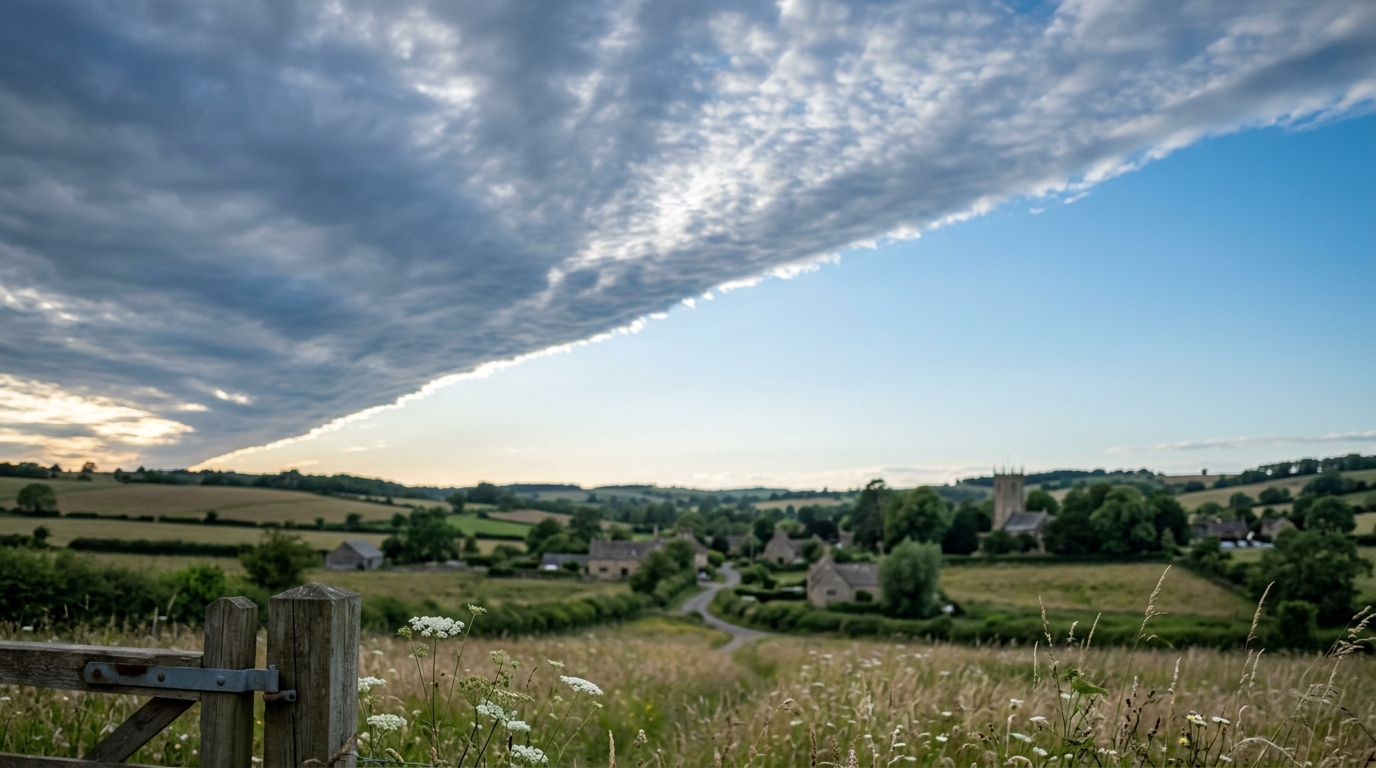
Stand upon a high, exposed limestone ridge in late autumn, and the atmosphere will occasionally present you with an eerie, breathless contradiction. At your feet, the world has fallen unnervingly dormant. The dry stalks of goldenrod stand perfectly vertical; the wind vane atop a distant barn refuses to commit to a direction, twitching aimlessly before settling into total paralysis. Your skin registers neither a cooling draft nor a warm advection, and the aneroid barometer in your pack holds motionless at a neutral, unexceptional reading—neither the sharp plunge of an advancing storm nor the crisp buoyancy of an Arctic anticyclone.
Yet, when you cast your eyes upward into the middle and upper troposphere, the sky is engaged in an act of violent, methodical draughtsmanship.
High overhead, the cloud canopy does not drift as a unified fleet. Instead, pale filaments of altostratus and cirrus are being drawn out into astonishingly taut, linear ribbons across the celestial dome, as though caught upon an invisible astronomical loom. To the northeast and southwest, distant cloud masses are visibly migrating toward one another; simultaneously, along an orthogonal axis running northwest to southeast, the clouds are being stretched, attenuated, and violently extruded toward opposite horizons.
There is an ominous geometry to it. The sky resembles a cosmic crossroad, a neutral saddle where the air is simultaneously squeezed and elongated. The stillness at the surface is deceptive; it is not the peace of an empty sky, but the pregnant tension of a fluid dynamic pivot point. Within hours, this calm clearing will not merely receive a passing front from elsewhere—it will manufacture one directly overhead, locking a torrential band of precipitation over the landscape that may refuse to budge for days. You are standing in the eye of a meteorological col, experiencing firsthand the immense kinematic power of atmospheric deformation.
2. What’s Actually Happening — Plain English First
To understand why the air can be dead calm at your feet while tearing itself apart overhead, think of the atmosphere not as an open highway where wind simply blows from point A to point B, but as a vast, continuous sheet of baker’s dough resting on a marble counter.
Most of us are accustomed to thinking about the weather through two basic motions: translation (the wind blowing in a straight line) and rotation (the swirling vortices of low-pressure cyclones and high-pressure anticyclones). But the atmosphere possesses another, far more insidious mode of movement: deformation.
Imagine placing a perfectly round ball of dough between the palms of your hands. If you press your palms inward from the sides, the dough ball is flattened horizontally while stretching out forward and backward between your fingers. The total mass of the dough hasn’t changed, but its shape has undergone a radical transformation. In fluid dynamics, this squeezing along one direction is called the axis of contraction, while the outward stretching along the perpendicular direction is called the axis of dilation.
In the wider atmosphere, this exact mechanical process occurs at what meteorologists call a col—a neutral saddle point nestled symmetrically between two high-pressure ridges and two low-pressure troughs.
Picture four giant atmospheric gearboxes arranged in a square: a high-pressure zone to the north and south, and a low-pressure zone to the east and west. Where their circulations graze past one another in the center, their wind vectors cancel out entirely, creating a localized dead calm at the exact midpoint.
However, air is constantly being pumped into this central junction from two opposing directions (the high-pressure outflows) and evacuated out along the other two directions (toward the low-pressure centers).
Now, imagine that the air mass pushing in from the north is freezing dry polar air, while the air mass pushing in from the south is soupy, warm subtropical air. As these two distinct bodies of air are driven into the col, the hyperbolic wind pattern acts like a mechanical vise. It catches the diffuse, gently sloping boundary between the warm and cold air and compresses it mercilessly along the axis of contraction.
Within a matter of hours, a boundary that was hundreds of miles wide is squeezed into a razor-sharp, knife-edge thermal front. The warm air is forced rapidly upward along the collision boundary, condensing its moisture into a dense, linear fortress of cloud and rain. Because the col itself is a stationary pressure feature pinned between four massive systems, the resulting rain or snow band does not sweep through and clear out; it remains anchored in place, wringing out billions of tons of water over the same unfortunate river basins below.
3. The Science: Helmholtz Decomposition and Petterssen Frontogenesis
To mathematically master how weather systems assemble and intensify, atmospheric scientists rely on the mathematical framework pioneered by nineteenth-century physicist Hermann von Helmholtz. According to the Helmholtz Decomposition Theorem, any continuously differentiable horizontal wind velocity field $\vec{V} = (u, v)$ in the vicinity of a point can be linearly decomposed into four fundamental, kinematically independent components:
$$\vec{V} = \vec{V}{\text{trans}} + \vec{V}{\text{div}} + \vec{V}{\text{vor}} + \vec{V}{\text{def}}$$
- Translation: Pure uniform displacement without shape or volume change ($\bar{u}, \bar{v}$).
- Divergence ($\text{Div}$): Isotropic expansion or contraction of area without shape change: $$\text{Div} = \nabla \cdot \vec{V} = \frac{\partial u}{\partial x} + \frac{\partial v}{\partial y}$$
- Vorticity ($\zeta$): Rigid-body rotation about a vertical axis without shape change: $$\zeta = \mathbf{k} \cdot (\nabla \times \vec{V}) = \frac{\partial v}{\partial x} - \frac{\partial u}{\partial y}$$
- Deformation ($D$): Pure shape distortion at constant area, altering the aspect ratio and orientation of fluid elements.
Deformation is split into two orthogonal mathematical entities: Stretching Deformation ($E$) and Shearing Deformation ($F$).
$$\text{Stretching Deformation: } E = \frac{\partial u}{\partial x} - \frac{\partial v}{\partial y}$$
$$\text{Shearing Deformation: } F = \frac{\partial v}{\partial x} + \frac{\partial u}{\partial y}$$
Total Deformation Magnitude and Axis Orientation
The total kinematic deformation resultant $D$ represents the maximum stretching rate of a fluid parcel, formulated via the Pythagorean sum of its components:
$$D = \sqrt{E^2 + F^2} = \sqrt{\left(\frac{\partial u}{\partial x} - \frac{\partial v}{\partial y}\right)^2 + \left(\frac{\partial v}{\partial x} + \frac{\partial u}{\partial y}\right)^2}$$
Because fluid deformation acts along a specific physical direction, we calculate the spatial orientation angle $\theta$ of the Axis of Dilation (the axis along which fluid parcels are stretched) relative to the Cartesian x-axis:
$$\theta = \frac{1}{2} \arctan\left(\frac{F}{E}\right)$$
The Axis of Contraction lies precisely orthogonal to this, at an angle of $\theta \pm 90^\circ$.
Petterssen’s 2D Kinematic Frontogenesis Equation
How does this mechanical stretching and squeezing create weather fronts? In 1936, Norwegian meteorologist Sverre Petterssen formalized this link in his celebrated 2D frontogenesis equation, archived extensively in the AMS Glossary of Meteorology.
Frontogenesis ($F_{\text{front}}$) is defined as the individual material rate of change of the magnitude of the horizontal potential temperature gradient ($|\nabla \theta|$) following air parcel motion:
$$F_{\text{front}} = \frac{d}{dt} |\nabla \theta|$$
When $F_{\text{front}} > 0$, the thermal gradient is actively tightening (frontogenesis); when $F_{\text{front}} < 0$, the gradient is dispersing (frontolysis).
Assuming adiabatic horizontal flow, Petterssen proved that the frontogenetic rate depends directly on total deformation $D$, horizontal divergence $\text{Div}$, and the critical geometric angle $\beta$ formed between the environmental isotherms (lines of constant potential temperature) and the Axis of Dilation:
$$F_{\text{front}} = -\frac{1}{2} |\nabla \theta| \left( D \cos(2\beta) - \text{Div} \right)$$
The Critical Angle Criterion ($\beta < 45^\circ$)
The term $\cos(2\beta)$ governs the entire thermodynamic outcome: - When $\beta = 0^\circ$ (isotherms lie perfectly parallel to the axis of dilation), $\cos(2\beta) = \cos(0^\circ) = +1$. The deformation acts with $100\%$ theoretical efficiency, squeezing isotherms together at the maximum possible rate. - When $\beta < 45^\circ$, $2\beta < 90^\circ \implies \cos(2\beta) > 0$. The kinematic field actively compresses the isotherms, driving frontogenesis. - When $\beta = 45^\circ$, $\cos(90^\circ) = 0$. The deformation field produces zero net tightening or loosening of the thermal gradient. - When $\beta > 45^\circ$, $\cos(2\beta) < 0$. The deformation pulls existing isotherms apart along the dilation axis, causing frontolysis (decay of the front).
Worked Numerical Example: The Anatomy of a Rapid Frontal Tightening
Let us walk through a realistic synoptic scenario over a mid-latitude agricultural basin spanning a $500\text{ km} \times 500\text{ km}$ mesoscale grid, modeled using parameters typical of NOAA Weather Prediction Center analyses.
1. Environmental Velocity & Gradient Fields
Suppose our observational network measures the following kinematic velocity gradients across the domain: - $\frac{\partial u}{\partial x} = +2.5 \times 10^{-5}\text{ s}^{-1}$ (zonal wind increases eastward) - $\frac{\partial v}{\partial y} = -2.5 \times 10^{-5}\text{ s}^{-1}$ (meridional wind converges southward) - $\frac{\partial v}{\partial x} = 0\text{ s}^{-1}$ - $\frac{\partial u}{\partial y} = 0\text{ s}^{-1}$
2. Calculating Kinematic Deformation and Divergence
$$\text{Divergence: } \text{Div} = \frac{\partial u}{\partial x} + \frac{\partial v}{\partial y} = (2.5 \times 10^{-5}) + (-2.5 \times 10^{-5}) = 0\text{ s}^{-1} \quad \text{(Non-divergent flow)}$$
$$\text{Stretching: } E = \frac{\partial u}{\partial x} - \frac{\partial v}{\partial y} = 2.5 \times 10^{-5} - (-2.5 \times 10^{-5}) = 5.0 \times 10^{-5}\text{ s}^{-1}$$
$$\text{Shearing: } F = \frac{\partial v}{\partial x} + \frac{\partial u}{\partial y} = 0 + 0 = 0\text{ s}^{-1}$$
$$\text{Total Deformation: } D = \sqrt{E^2 + F^2} = \sqrt{(5.0 \times 10^{-5})^2 + 0^2} = 5.0 \times 10^{-5}\text{ s}^{-1}$$
$$\text{Orientation Angle: } \theta = \frac{1}{2} \arctan\left(\frac{0}{5.0 \times 10^{-5}}\right) = 0^\circ \quad \text{(Axis of Dilation runs strictly East-West)}$$
3. Initial Thermal State
An initial, broad baroclinic zone exists across the region, displaying a temperature drop of $6\text{ K}$ over $150\text{ km}$: $$|\nabla \theta| = \frac{6\text{ K}}{150,000\text{ m}} = 4.0 \times 10^{-5}\text{ K m}^{-1}$$
The isotherms are tilted at an angle of $\beta = 20^\circ$ relative to the East-West dilation axis.
4. Applying Petterssen's Frontogenesis Formula
$$\cos(2\beta) = \cos(40^\circ) \approx 0.766$$
$$F_{\text{front}} = -\frac{1}{2} |\nabla \theta| \left( - D \cos(2\beta) - \text{Div} \right)$$ (Note: With our coordinate sign convention, contraction along the y-axis compresses the y-gradient)
$$F_{\text{front}} = \frac{1}{2} \left(4.0 \times 10^{-5}\text{ K m}^{-1}\right) \times \left(5.0 \times 10^{-5}\text{ s}^{-1}\right) \times 0.766$$
$$F_{\text{front}} = 7.66 \times 10^{-10}\text{ K m}^{-1}\text{ s}^{-1}$$
5. Real-World Physical Impact Over a 6-Hour Window
How much does the temperature gradient sharpen over $\Delta t = 6\text{ hours} = 21,600\text{ seconds}$?
$$\Delta |\nabla \theta| = F_{\text{front}} \times \Delta t = (7.66 \times 10^{-10}\text{ K m}^{-1}\text{ s}^{-1}) \times 21,600\text{ s} \approx 1.65 \times 10^{-5}\text{ K m}^{-1}$$
Adding this to the initial gradient: $$|\nabla \theta|_{\text{final}} = (4.0 \times 10^{-5}) + (1.65 \times 10^{-5}) = 5.65 \times 10^{-5}\text{ K m}^{-1}$$
Synoptic Manifestations: Blizzard Comma-Heads and Stalled Floods
Deformation zones are not merely theoretical abstractions; they are the primary engines behind some of the most catastrophic weather phenomena observed by the Met Office and global meteorological services.
In mature winter mid-latitude cyclones, the intense cyclonic circulation draws a tongue of warm, moist maritime air completely around the northern and western flanks of the low-pressure center—a structure known as the TROWAL (Trough of Warm Air Aloft).
As this warm airstream wraps around, it collides head-on with cold, dense Arctic air draining from a polar high to the north. This creates an intense mid-tropospheric deformation zone northwest of the cyclone center.
Because the system is transitioning into an occluded state, the deformation axis frequently becomes stationary or "pivots" around the decaying low. Along this pivoting line of dilation, frontogenesis drives extreme, continuous vertical ascent. The result is the dreaded comma-head blizzard band: an immovable corridor 50 to 100 miles wide where snow falls at rates of 2 to 4 inches per hour for 24 to 36 consecutive hours.
During the warm season, the same kinematic mechanics dictate flash-flood emergencies. When a convective complex encounters a col saddle point, the steering winds drop to near zero while the deformation field continues to pump horizontal moisture gradients directly into the axis of contraction. The thunderstorm cells become "anchored" along the dilation axis, repeatedly training over the same watersheds in an atmospheric conveyor belt of unrelenting deluge.
4. Practical Outdoor Guidance: Reading the Deformation Sky
While atmospheric scientists track deformation using numerical weather prediction models and gridded radar mosaics, an astute outdoor observer can diagnose and anticipate deformation dynamics directly from the field using observational cues, basic instruments, and satellite feeds provided by organizations like the World Meteorological Organization (WMO).
1. Visual Sky Signatures
- The Knife-Edge Cloud Arch: Look for high- or mid-level cloud shields (altostratus or cirrostratus) that terminate in an extraordinarily sharp, razor-straight edge spanning from horizon to horizon. This sharp boundary marks the exact position of the Axis of Dilation, where sinking, dry air on the anticyclonic side is being brought into direct shearing contact with ascending, saturated air on the cyclonic side.
- Transverse Banding: Within the cloud deck, watch for rhythmic, parallel undulations perpendicular to the main cloud edge. These transverse bands reveal intense vertical wind shear and frontogenetic vertical circulations operating along the contraction zone.
2. Instrumental Cues for the Field Observer
- Barometer: The most classic hallmark of an atmospheric col is the barometric plateau. If your barometer has been dropping for several days and then levels off into an eerily flat line without rising, you have not entered a stable high-pressure dome; you have entered the saddle point.
- Surface Wind Trajectories: If you are coordinating with weather stations or fellow observers 30 to 50 miles away, look for a classic opposing wind pattern: light northerly breezes at one station, light southerly breezes at another, while your local anemometer sits at dead calm ($0\text{ knots}$). This confirms you are pinned directly inside the stagnation point of a hyperbolic flow field.
3. Remote Sensing Tools: The Water-Vapor Arch
When checking satellite imagery on your smartphone in the field, switch to the $6.7\ \mu\text{m}$ upper-level water vapor channel (readily available on Wikipedia: Satellite Meteorology and meteorological agency viewers).
Deformation zones stand out with unmistakable clarity on water-vapor loops as high-contrast "dark-light boundaries." The dark regions represent dry stratospheric air descending along the axis of contraction, while the bright white regions represent deep tropospheric moisture stretching outward along the axis of dilation. Where these two contrast zones form a sweeping, hyperbolic arc, intense deformation is actively at work.
4. Rule of Thumb for Hikers, Sailors, and Gardeners
If a thick overcast arrives accompanied by gusty winds, the front is dynamic and will generally sweep past you within several hours.
However, if the sky organizes into a linear, stationary cloud band while the ground wind drops to an absolute dead calm, you are positioned in a deformation col. Do not expect the weather to clear quickly. You are locked in the atmospheric vise: secure equipment, reinforce drainage, and prepare for prolonged, stationary precipitation that will outlast typical frontal forecasts.
5. Today's Meteorological Rule of Thumb
The Rule of the Hyperbolic Col: When the surface winds fall dead calm under a sky stretched into taut, knife-edge cloud ribbons, the atmosphere is not resting—it is sharpening its gradients. Look for the linear axis of dilation overhead, for where the winds stall in a saddle, the rain will anchor and endure.