Radar Bright Band & Melting Layer Dynamics: How Dielectric Transitions and Ice Aggregation Forge Stratiform Reflectivity Peaks
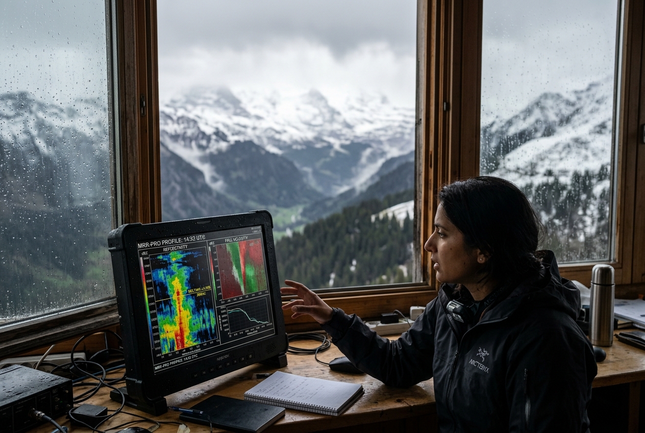
Under a slate-grey November sky in a sub-alpine valley, the physical reality of the atmosphere often presents a tranquil, almost monotonous face. A pedestrian stepping outside feels a damp, penetrating chill as the thermometer lingers motionless at $3^\circ\text{C}$. A uniform blanket of low nimbostratus clouds obscures the surrounding peaks, releasing nothing more threatening than a steady, dreary drizzle. The rhythmic patter of small drops—scarcely two millimetres across—coats the pavement with a glassy sheen, accompanied by the earthy scent of petrichor rising from cold, saturated soil. The barometric pressure drifts downward in a gentle, predictable curve; the air is calm, save for an intermittent, sluggish breeze.
Yet, opening a high-resolution smartphone weather application reveals a startlingly contradictory image. Directly overhead, where the observer stands enveloped in gentle drizzle, the radar display blazes with an ominous core of crimson and magenta echoes. On the standard operational reflectivity scale, these colours signify severe convective fury: returns exceeding $50\text{ dBZ}$, typically indicative of torrential summer cloudbursts, severe urban flash flooding, or destructive hail.
================================================================================
VERTICAL RADAR BEAM CROSS-SECTION THROUGH A STRATIFORM PRECIPITATION COLUMN
================================================================================
 Altitude
    ^
    |  [PRISTINE ICE & SNOW]       Dry aggregate snowflakes: D ~ 3-8 mm
    |  T < 0°C                     Low dielectric factor (|K|^2 ≈ 0.19)
    |                              Fall velocity: v_t ≈ 1.0 m/s
    |                              Reflectivity: Z ≈ 20 - 30 dBZ
----+--------------------------------------------------------------------------- <--- 0°C Melting Level
    |  [STAGE 1: AGGREGATION]      Sticky collision -> Giant snowflakes (D > 15 mm)
    |  [STAGE 2: WATER COATING]    Liquid veneer forms -> Dielectric surge (|K|^2 -> 0.93)
    |                              *********************************************
    |  MELTING LAYER               *** PEAK RADAR BRIGHT BAND (Z ≈ 45 - 55 dBZ) ***
    |  (100 - 300 m depth)         *********************************************
    |  [STAGE 3: COLLAPSE]         Surface tension collapses snowflake -> Raindrop
    |  [STAGE 4: ACCELERATION]     Velocity jump: v_t -> 7.0 m/s (Flux dilution)
----+--------------------------------------------------------------------------- <--- Complete Melting
    |  [LIQUID RAINFALL]           Compact raindrops: D ~ 1 - 2.5 mm
    |  T > 0°C                     High fall speed, diluted spatial concentration
    |                              Reflectivity plummets: Z ≈ 25 - 32 dBZ
    v                              Ground reality: Monotonous light rain / drizzle
================================================================================
This striking discrepancy between the quiet drizzle on the ground and the apparent violent storm aloft is not an electronic glitch or instrument calibration failure. It is the signature manifestation of one of the most elegant and fundamental phenomena in observational meteorology: the radar bright band. Governed by the thermodynamic and microphysical transitions of hydrometeors crossing the zero-degree isotherm, this elevated horizontal layer of amplified radar backscatter acts as an optical and electromagnetic illusion. Understanding its mechanics requires dissecting the dielectric properties of water, the mathematics of microwave backscattering, and the hydrodynamic evolution of snowflakes as they collapse into rain.
1. What Is Happening: The Intuitive Physics of the Melting Layer
To understand why a gentle shower appears on radar as a violent tempest, we must picture the troposphere not as a static reservoir of air, but as a dynamic thermodynamic processing column. In stratiform precipitation systems—wide, steady cloud shields formed along warm fronts or within decaying low-pressure systems—precipitation universally originates high above our heads as delicate ice crystals.
Think of dry snow falling through the upper atmosphere as a drifting collection of fluffy, intricate down feathers. Because ice crystals at temperatures well below freezing are cold and dry, they bounce off one another upon collision, maintaining modest dimensions. As these snowflakes descend into warmer air, they eventually cross the melting level—the altitude where the ambient atmospheric temperature warms past $0^\circ\text{C}$ ($32^\circ\text{F}$).
[Dry Ice Crystal]  -->  [Sticky Aggregate]  -->  [Water-Coated Giant]  -->  [Compact Raindrop]
   (Cold / Rigid)        (0°C Surface Film)       (Dielectric Water Shell)       (Rapid Fall / Diluted)
The moment a snowflake enters air above freezing, its delicate outer extremities begin to liquefy, coating the ice matrix in a microscopic film of meltwater. This thin coating fundamentally alters the physics of the descent in two consecutive ways:
- The Stickiness Factor: Wet ice is extraordinarily sticky. Instead of rebounding, colliding snowflakes fuse together into sprawling, multi-branched aggregate clusters—giant, porous snowflakes that can span several centimetres across.
- The Microwave Chameleon Effect: Microwave weather radar does not possess X-ray vision; it cannot perceive what lies at the core of a particle. Because liquid water interacts with electromagnetic waves nearly five times more strongly than solid ice, the radar beam strikes this sprawling aggregate, detects the liquid film on its exterior, and misinterprets the entire multi-centimetre aggregate snowflake as a gigantic, solid raindrop.
Because radar backscattering is exponentially sensitive to particle diameter, this hybrid particle—possessing the enormous physical dimensions of an aggregate snowflake combined with the electromagnetic reflectivity of liquid water—reflects an immense surge of microwave energy back to the radar antenna.
Moments later, as the snowflake continues its descent through warmer air, surface tension forces the melted structure to collapse inward, condensing the sprawling fractal into a compact, spherical raindrop only a fraction of its former diameter. Simultaneously, the streamlined drop accelerates, falling five to eight times faster than the parent snowflake. This acceleration stretches out the vertical spacing between drops, diluting their spatial concentration. Consequently, beneath this narrow melting zone, the returned radar power plummets back to modest values, aligning once again with the mild rain experienced by the observer on the ground.
2. Electromagnetic Foundations: Rayleigh Scattering and Dielectric Physics
To transition from conceptual intuition to quantitative atmospheric physics, we examine how microwave radiation interacts with hydrometeors within the framework of electromagnetic scattering theory established by Rayleigh Scattering in Radar Meteorology.
Operational meteorological radars—such as the S-band ($\lambda \approx 10\text{ cm}$) systems deployed across the NOAA National Weather Service Radar Network and C-band ($\lambda \approx 5.6\text{ cm}$) radars utilized throughout the Met Office Radar Network—operate primarily within the Rayleigh scattering regime. This condition is valid whenever the particle diameter $D$ is substantially smaller than the incident radar wavelength $\lambda$ (conventionally $D < \lambda / 16$).
Under the Rayleigh approximation, the backscattering cross-section $\sigma_b$ of an individual spherical hydrometeor of physical diameter $D$ is formulated as:
$$\sigma_b = \frac{\pi^5}{\lambda^4} |K|^2 D^6$$
where: - $\lambda$ represents the radar operating wavelength (metres). - $D$ is the hydrometeor diameter (metres). - $|K|^2$ is the dimensionless dielectric factor of the scattering medium.
The dielectric factor $|K|^2$ quantifies the polarizability of the hydrometeor material when subjected to the oscillating electric field of the radar pulse. It is defined through the complex relative permittivity $\epsilon_r = \epsilon' - j\epsilon''$ as:
$$|K|^2 = \left| \frac{\epsilon_r - 1}{\epsilon_r + 2} \right|^2$$
Herein lies the physical origin of the bright band. The molecular structure of liquid water allows its permanent electric dipoles to rotate freely in response to microwave frequencies, yielding a very high relative permittivity ($\epsilon_{r,\text{water}} \approx 80$ at $0^\circ\text{C}$). Conversely, in solid ice, the water molecules are locked into a crystalline hexagonal lattice that impedes dipole reorientation at gigahertz frequencies ($\epsilon_{r,\text{ice}} \approx 3.17$).
Computing the respective dielectric factors at microwave frequencies near $0^\circ\text{C}$ reveals:
$$|K_w|^2 = \left| \frac{80 - 1}{80 + 2} \right|^2 \approx \left( \frac{79}{82} \right)^2 \approx 0.928 \approx 0.93$$
$$|K_i|^2 = \left| \frac{3.17 - 1}{3.17 + 2} \right|^2 \approx \left( \frac{2.17}{5.17} \right)^2 \approx 0.176 - 0.197$$
================================================================================
DIELECTRIC FACTOR RATIO & BACKSCATTER POWER GAIN
================================================================================
Ratio:                |K_w|^2 / |K_i|^2 = 0.93 / 0.18 ≈ 5.17
Logarithmic Gain:     10 * log10(5.17) ≈ +7.13 dBZ
Physical Consequence: A snowflake acquiring a micro-thin water skin enhances its
                      radar backscatter by > 500% before its diameter changes!
================================================================================
Summing the contributions over an atmospheric sample volume containing a particle size distribution $N(D)$, the equivalent radar reflectivity factor $Z_e$ (conventionally expressed in units of $\text{mm}^6/\text{m}^3$) is defined as:
$$Z_e = \frac{|K|^2}{|K_w|^2} \int_0^\infty N(D) D^6 \, dD$$
Because radar meteorology conventionally benchmarks all reflectivity calculations against the dielectric constant of liquid water ($|K_w|^2 = 0.93$), the un-melted dry ice region above the freezing level exhibits an inherently depressed reflectivity:
$$Z_{\text{dry snow}} = \frac{|K_i|^2}{|K_w|^2} \sum N(D) D^6 \approx 0.20 \sum N(D) D^6$$
The moment a snowflake develops an ultra-thin outer sheath of liquid water, its dielectric factor transitions discontinuously from $|K_i|^2 \approx 0.18$ to $|K_w|^2 \approx 0.93$. This single dielectric phase shift produces an immediate $+7.13\text{ dB}$ surge in returned radar power, completely independent of any microphysical changes in particle size.
3. The Microphysics of the Four-Stage Melting Sequence
The evolution of stratiform precipitation through the melting layer is a cascade of four distinct, coupled microphysical stages occurring across a vertical depth of approximately 200 to 500 metres.
Stage 1: Sticky Aggregation  ---> Stage 2: Dielectric Peak ---> Stage 3: Surface Tension Collapse ---> Stage 4: Velocity Dilution
(D expands up to 20 mm)          (Water shell on giant core)    (D collapses: 15 mm -> 2 mm)           (v_t jumps: 1 m/s -> 8 m/s)
Stage 1: Incipient Melting & Sticky Aggregation
As pristine dendritic crystals descend through the $0^\circ\text{C}$ isotherm (defined in the AMS Glossary of Meteorology), their intricate crystal tips begin to melt. This forms a quasi-liquid surface layer that dramatically amplifies the collection efficiency and collision stickiness coefficient $\alpha(T)$ of the hydrometeors.
Collisions between falling snowflakes no longer result in elastic bouncing or mechanical fracturing; instead, the wet ice surfaces bond instantaneously. Over a vertical descent of 50 to 150 metres below the $0^\circ\text{C}$ level, stellar dendrites aggregate into massive, low-density fluffy aggregates with equivalent diameters expanding from $D \approx 2\text{--}5\text{ mm}$ to $D \gg 15\text{--}25\text{ mm}$. Because radar backscattering scales with the sixth power of the diameter ($D^6$), this rapid geometric expansion sets the stage for a dramatic increase in reflectivity.
Stage 2: Dielectric Transformation (The Reflectivity Zenith)
As melting progresses, meltwater percolates through the porous ice lattice and coats the outer perimeter of the aggregate. In accordance with the Maxwell Garnett and Bohren-Battan effective medium theories for mixed-phase dielectric spheres, when the continuous outer matrix of an inclusion is composed of the higher-permittivity substance (water), the effective dielectric constant of the entire composite particle approaches that of pure water.
The radar pulse encounters a particle with the immense physical cross-section of a multi-centimetre aggregate snowflake ($D \approx 15\text{--}20\text{ mm}$) behaving electromagnetically as if it were pure liquid water. The confluence of maximal aggregation ($D^6$) and the fully activated dielectric factor ($|K_w|^2 \approx 0.93$) produces the bright band's peak reflectivity: a narrow zone where $Z$ surges $+5\text{ to }+15\text{ dBZ}$ above the pristine snowfall above, frequently exceeding $50\text{ to }55\text{ dBZ}$.
Stage 3: Hydrodynamic Collapse and Shrinkage
The aggregate cannot sustain this bloated state. As the structural ice framework within the snowflake melts beyond a critical liquid water fraction ($f_w > 0.5\text{--}0.7$), internal capillary forces and surface tension rapidly pull the sprawling, air-filled matrix inward. The hollow, low-density aggregate collapses into a single, compact, high-density spherical or oblate raindrop.
This collapse triggers a severe reduction in particle diameter:
Mass Conservation during Collapse:
m_aggregate = m_drop  ==>  ρ_snow * (π/6) * D_snow^3 = ρ_water * (π/6) * D_drop^3
Given that the bulk density of an uncompacted aggregate snowflake is approximately $\rho_{\text{snow}} \approx 0.05\text{ g/cm}^3$ while liquid water is $\rho_{\text{water}} = 1.0\text{ g/cm}^3$, the diameter ratio is:
$$\frac{D_{\text{drop}}}{D_{\text{snow}}} = \left( \frac{\rho_{\text{snow}}}{\rho_{\text{water}}} \right)^{1/3} = (0.05)^{1/3} \approx 0.368$$
Applying the Rayleigh $D^6$ backscattering dependency to this collapse reveals an enormous reduction in radar cross-section:
$$\left(\frac{D_{\text{drop}}}{D_{\text{snow}}}\right)^6 = (0.368)^6 \approx 0.0025$$
This physical shrinkage alone suppresses the hydrometeor's individual radar backscatter by a factor of 400 (a decrease of $-26\text{ dB}$).
Stage 4: Kinematic Velocity Dilution and Mass Flux Continuity
Simultaneously, the aerodynamic drag characteristics of the hydrometeor change fundamentally. A sprawling, low-density snowflake possesses a large surface-area-to-mass ratio, yielding a low terminal fall speed governed by:
$$v_{\text{snow}} \approx 0.8\text{ to }1.2\text{ m/s}$$
Upon collapsing into a streamlined, high-density liquid drop, the terminal fall velocity increases dramatically according to empirical terminal velocity relations (such as Gunn-Kinzer or Atlas-Ulbrich formulations):
$$v_{\text{rain}} \approx 9.65 - 10.3 \exp(-0.6 D) \approx 6.0\text{ to }9.0\text{ m/s}$$
================================================================================
KINEMATIC FLUX CONSERVATION & NUMBER DENSITY DILUTION
================================================================================
Steady-State Vertical Mass Flux:
    Flux (Φ) = N * v_t * m = Constant

Since mass (m) is conserved per hydrometeor:
    N_snow * v_snow = N_rain * v_rain

Solving for Raindrop Number Density (N_rain):
    N_rain = N_snow * (v_snow / v_rain)

Given v_snow ≈ 1.0 m/s and v_rain ≈ 7.5 m/s:
    N_rain ≈ N_snow * (1.0 / 7.5) ≈ 0.133 * N_snow
================================================================================
Because the raindrops fall roughly 7.5 times faster than their parent snowflakes, they evacuate the lower boundary of the melting layer far more rapidly than they entered it from above. The spatial number concentration of particles per cubic metre of air ($N$) drops by over $85\%$.
Because total reflectivity factor $Z = \sum N(D) D^6$ depends linearly on particle concentration $N$, this kinematic dilution reduces reflectivity by an additional factor of 7.5:
$$\Delta Z_{\text{velocity}} = 10 \log_{10}\left(\frac{v_{\text{snow}}}{v_{\text{rain}}}\right) = 10 \log_{10}\left(\frac{1.0}{7.5}\right) \approx -8.75\text{ dB}$$
Combining the hydrodynamic collapse ($-26\text{ dB}$) and velocity dilution ($-8.75\text{ dB}$) against the dielectric gain ($+7.13\text{ dB}$) explains why reflectivity immediately below the bright band plummets by 15 to 25 dBZ relative to the bright band peak, settling into the familiar 25–35 dBZ echoes characteristic of light-to-moderate stratiform rainfall.
4. Dual-Polarization Radar Diagnostics
Modern operational meteorological networks, including the dual-polarization WSR-88D fleet governed by the World Meteorological Organization (WMO) observational standards, do not rely solely on single-polarization horizontal reflectivity ($Z_h$) to detect melting layers. Dual-polarization radar transmits and receives pulses in both horizontal ($H$) and vertical ($V$) polarizations, providing critical microphysical insights into particle shape, orientation, and thermodynamic phase diversity.
Height (km)
   ^
4.0|         \  Z_h Profile           |  Z_dr Profile         |  ρ_hv Profile
   |          \                       |                       |
3.0|           \                      |                       |
   |            \                     |                       |  0°C Isotherm
---+-------------*--------------------+-----------------------+--- ----------
2.5|              \                   |                      /
   |               \ [BRIGHT BAND]    |   [Z_dr BULGE]      /  [ρ_hv DIP]
2.0|               / (45-55 dBZ)      |   (+1.5 to +3.5 dB)/   (0.85 - 0.92)
   |              /                   |                   /
---+-------------*--------------------+------------------+-------------------
1.5|            /                     |                  |
   |           /  Rainfall            |  Rainfall        |  Pure Rain
1.0|          /   (25-30 dBZ)         |  (0.2 - 0.8 dB)  |  (> 0.98)
   v
The Copolar Correlation Coefficient ($\rho_{hv}$)
The copolar correlation coefficient $\rho_{hv}$ measures the statistical consistency between the horizontal and vertical backscattered power and phase across consecutive radar pulses within a pulse volume:
$$\rho_{hv} = \frac{\langle s_{hh} s_{vv}^* \rangle}{\sqrt{\langle |s_{hh}|^2 \rangle \langle |s_{vv}|^2 \rangle}}$$
- In pure rain, drops are uniformly oriented, oblate spheroids, yielding $\rho_{hv} > 0.98$.
- In pristine dry snow aloft, ice crystals exhibit homogeneous dielectric properties, maintaining $\rho_{hv} \approx 0.97\text{--}0.99$.
- Within the melting layer, however, the radar pulse encounters a chaotic mixture of dry snowflakes, water-coated giant aggregates, tumbling asymmetric slush particles, and newly formed spherical raindrops. This extreme variance in particle shape, orientation, and complex dielectric permittivity causes $\rho_{hv}$ to dip sharply to characteristic values between $0.85$ and $0.94$. Operational hydrometeor classification algorithms identify this narrow depression in $\rho_{hv}$ as the definitive signature of the melting layer.
Differential Reflectivity ($Z_{dr}$)
Differential reflectivity is defined as the logarithmic ratio of horizontally to vertically polarized radar reflectivity factors:
$$Z_{dr} = 10 \log_{10}\left( \frac{Z_h}{Z_v} \right)$$
Because falling raindrops flatten aerodynamically into oblate spheroids with their broad axis oriented horizontally, $Z_{dr}$ serves as a direct indicator of particle shape and axis ratio.
Within the lower half of the bright band, large melting snowflakes exhibit an intense positive $Z_{dr}$ signature, frequently reaching $+1.5\text{ to }+3.5\text{ dB}$. As the aggregate melts, its aerodynamically compliant wet matrix flattens horizontally under relative wind shear while its water coating maximizes the horizontal dielectric cross-section ($Z_h \gg Z_v$).
Once full collapse occurs at the bottom of the melting layer, the resulting modest-sized raindrops ($D \approx 1\text{--}2\text{ mm}$) assume much more spherical shapes, causing $Z_{dr}$ to drop back to typical stratiform values of $+0.2\text{ to }+0.8\text{ dB}$.
5. Thermodynamic Feedbacks and Quantitative Precipitation Bias
The melting layer is not merely a passive recipient of environmental temperature; it actively modifies its thermodynamic environment through latent heat exchange.
================================================================================
THERMODYNAMIC COOLING VIA LATENT HEAT OF FUSION
================================================================================
Latent Heat of Fusion:        L_f = 3.34 x 10^5 J/kg
Specific Heat of Dry Air:     c_p = 1005 J/(kg·K)

Diabatic Column Cooling Rate Equation:
    (∂T / ∂t)_melting = - (L_f / c_p) * S_m

Where S_m is the melting rate of solid precipitation (kg of ice melted / kg of air / sec).
================================================================================
When snow melts into rain, it extracts latent heat of fusion directly from the surrounding air. Melting one kilogram of ice consumes $3.34 \times 10^5\text{ Joules}$ of thermal energy. In prolonged, moderate-to-heavy stratiform precipitation events, this continuous diabatic cooling cools the atmospheric layer immediately below the $0^\circ\text{C}$ isotherm.
Over several hours, if horizontal warm air advection is weak, this persistent cooling drives the atmospheric lapse rate within the melting layer toward an isothermal $0^\circ\text{C}$ state.
Initial Profile:      T(z) decreases linearly with height across 0°C level
Sustained Melting:    Diabatic cooling erodes temperature profile
Resulting State:      Thick Isothermal 0°C Layer forms -> Snow level descends hundreds of meters
This thermodynamic feedback forces the melting layer downward toward the ground, transforming cold rain into heavy wet snow at valley levels—a process known as the diabatic descent of the snow line, critical for alpine and transportation forecasting.
Quantitative Precipitation Estimation (QPE) Contamination
In radar hydrology, surface rainfall rate $R$ ($\text{mm/hr}$) is conventionally estimated from measured reflectivity $Z$ via empirical power-law relations such as the standard Marshall-Palmer Z-R Relationship:
$$Z = 200 R^{1.6} \implies R = \left( \frac{Z}{200} \right)^{1 / 1.6}$$
================================================================================
WORKED MATHEMATICAL EXAMPLE: BRIGHT BAND RADAR OVERESTIMATION
================================================================================
Scenario:
A weather radar beam intersects the melting layer at an altitude of 2.2 km.
The radar measures an uncorrected peak bright band reflectivity of Z = 52 dBZ.
At the surface, light stratiform rain is falling with an actual reflectivity of Z = 30 dBZ.

Step 1: Convert Reflectivities from dBZ to Linear mm^6/m^3:
    Z_linear = 10^(dBZ / 10)
    Z_measured = 10^(52 / 10) = 10^5.2 ≈ 158,489 mm^6/m^3
    Z_actual   = 10^(30 / 10) = 10^3.0 = 1,000 mm^6/m^3

Step 2: Calculate Rain Rate Predicted by Radar (R_radar):
    R_radar = (158,489 / 200)^(1 / 1.6)
    R_radar = (792.445)^0.625 ≈ 64.9 mm/hr  [TORRENTIAL DOWNPOUR / FLOOD WARNING]

Step 3: Calculate Actual Surface Rain Rate (R_actual):
    R_actual = (1,000 / 200)^(1 / 1.6)
    R_actual = (5.0)^0.625 ≈ 2.74 mm/hr     [GENTLE STRATIFORM DRIZZLE]

Step 4: Quantify the Estimation Error Factor:
    Error Factor = R_radar / R_actual = 64.9 / 2.74 ≈ 23.7x
================================================================================
If a radar algorithm samples the bright band aloft without applying a Vertical Profile of Reflectivity (VPR) correction, it interprets the 52 dBZ melting snow echo as an extreme torrential downpour of nearly $65\text{ mm/hr}$, overestimating the true ground precipitation ($2.74\text{ mm/hr}$) by a factor of nearly twenty-four. Operational hydrologic networks employ automated VPR identification algorithms to detect the bright band inflection points and normalize the radar beam's sampled volume down to realistic surface precipitation rates.
6. Practical Field Observations and Atmospheric Diagnostics
For outdoor professionals, mountaineers, hydrologists, and weather enthusiasts, understanding bright band dynamics provides actionable predictive power during stratiform weather events.
================================================================================
METEOROLOGICAL OBSERVER'S MELTING LAYER CHECKLIST
================================================================================
Surface Instrument        Reading / Trend             Microphysical Meaning
--------------------------------------------------------------------------------
Surface Thermometer       1.5°C to 4.0°C              Vulnerable to diabatic cooling
Wet-Bulb Temp (T_w)       <= 0.5°C                    Imminent rain-to-snow transition
Barometer                 Steady or slow fall         Stable stratiform dynamics
Wind Direction (Sfc)      Veering with height         Warm air advection counteracting cooling
Radar Dual-Pol (ρ_hv)     Depression to < 0.92        Exact altitude of active melting layer
Radar Dual-Pol (Z_dr)     Bulge to +2.0 dB            Base of melting layer / drop collapse zone
================================================================================
1. Estimating the Melting Layer Base via Surface Wet-Bulb Temperature
Raindrops and melting snowflakes experience evaporative cooling if the sub-cloud layer is unsaturated. Consequently, the true lower limit of the melting layer is governed not by the dry-bulb temperature ($T$), but by the wet-bulb temperature ($T_w$).
You can approximate the height of the melting layer base ($h_{\text{melt}}$, in metres above ground level) using surface dry-bulb temperature $T$ ($^\circ\text{C}$) and relative humidity $RH$ ($\%$) via the standard environmental lapse rate ($\Gamma \approx 6.5^\circ\text{C}/\text{km}$):
$$h_{\text{melt}} \approx \frac{T_w}{\Gamma} \times 1000 \approx \frac{T - \frac{100 - RH}{5}}{6.5} \times 1000$$
If surface $T = 4^\circ\text{C}$ and $RH = 85\%$:
$$T_w \approx 4 - \frac{15}{5} = 1.0^\circ\text{C} \implies h_{\text{melt}} \approx \frac{1.0}{6.5} \times 1000 \approx 154\text{ metres AGL}$$
A mountain hiker climbing only 160 metres will cross directly out of liquid rain, pass through the sticky bright-band aggregate zone, and encounter heavy, sticking snow.
2. Identifying Bright Band Contamination on Public Radars
When inspecting public radar imagery during widespread winter or spring precipitation: - Look for a persistent, stationary ring or curved band of elevated reflectivity ($40\text{--}50\text{ dBZ}$) that mirrors the radar site at a constant radial distance. - Because a radar scans at fixed elevation angles (e.g., $0.5^\circ, 1.5^\circ$), its conical beam rises with range. A horizontal melting layer at 2,000 metres altitude will be intersected by the $0.5^\circ$ beam at a ground range of approximately $R \approx 2000 / \sin(0.5^\circ) \approx 230\text{ km}$, creating a concentric halo of intense reflectivity that does not correspond to any genuine cloudburst on the ground.