Brewer-Dobson Circulation & Stratospheric Wave Drag: How Planetary Wave Breaking and Downward Control Drive Global Ozone Transport
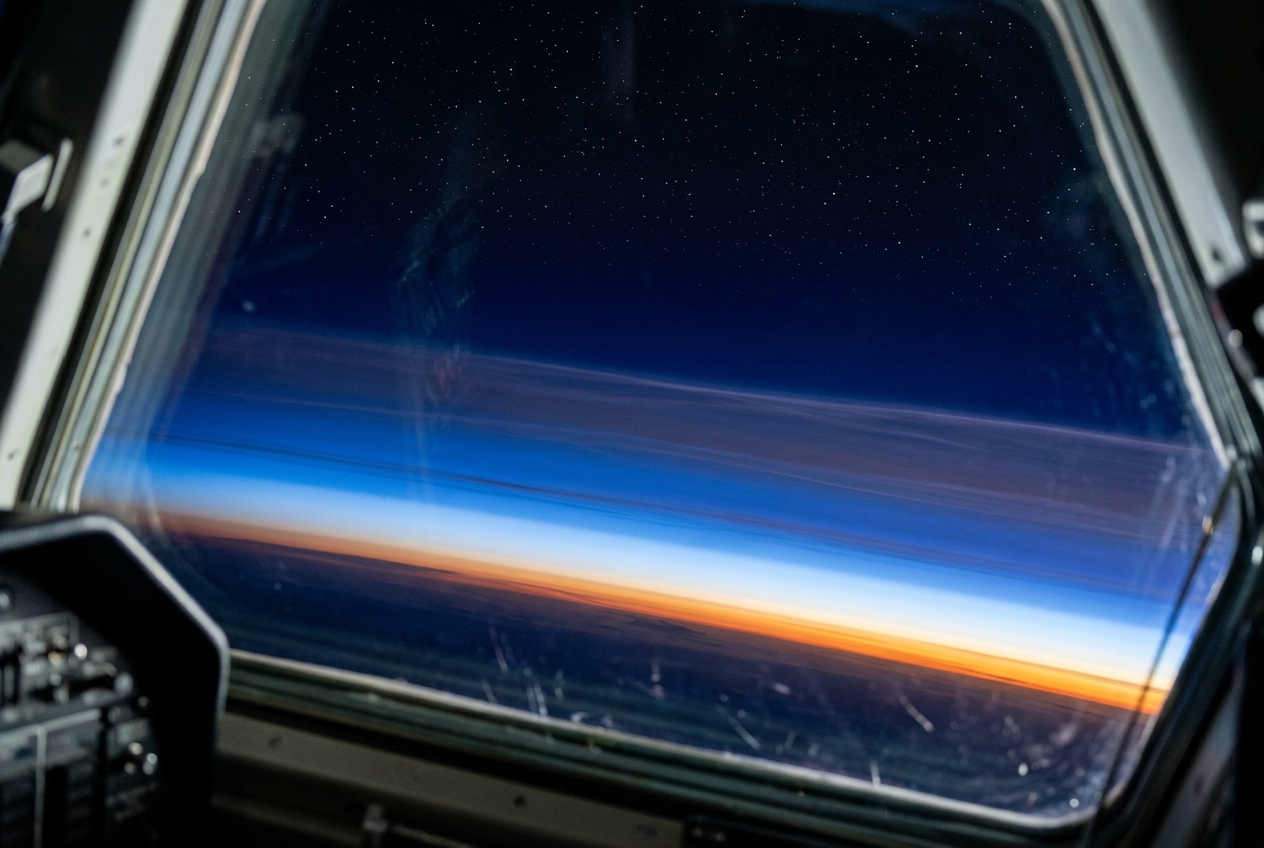
The Blue Hour and the Silent Sky
Stand on an exposed North Atlantic headland in late March just after the sun has slipped beneath the horizon. The coastal gale that battered the headland through the afternoon has subsided into an eerie, glass-like calm. The air biting your cheeks is raw and dry, carrying an electric clarity that sharpens distant lighthouses against the twilight. If you tilt your head back, you will notice that the sky does not merely fade from orange to dusk; it passes through a narrow, breathtaking band of luminous, saturated sapphire—a deep, spectral indigo known to physicists as the Chappuis absorption band.
ALTITUDE
 (km)
  ^
50|                     STRATOPAUSE (Warm: ~0°C)
  |       . - ~ - .                      . - ~ - .
  |     /           \                  /           \
30|    |  OZONE      |===============>| POLAR OZONE | (Spring Maximum)
  |    |  NURSERY    |    Deep Branch | ACCUMULATION|
  |     \ (Tropical)/                  \ (High-Lat) /
17|  ===\==========/====================\==========/=== TROPOPAUSE
  |      ^  Ascent                         |  Descent
  |      |  (TTL Cold Trap: -83°C)         v
 0|______|_________________________________|___________
     EQUATOR (0°)                      POLE (90°N/S)
At this exact moment, you are breathing air that has been shaped by events occurring twenty kilometres above your head in the absolute darkness of the middle stratosphere. The barometric pressure at your feet sits at a resolute 1,028 hectopascals, yet the crystal stillness of the evening is the ground-level exhaust of a planetary heat engine. Far above the tropospheric weather—above the cirrus sheets, above the cruise altitude of commercial jetliners—a vast, silent overturning circulation is drawing millions of tonnes of air out of the equatorial tropics, hoisting it through an unearthly deep-freeze, driving it across thousands of miles of latitude, and pushing it inexorably downward toward the pole.
This is the Brewer-Dobson Circulation. It is the global conveyor belt of the middle atmosphere: a wave-driven suction pump that freeze-dries the sky, redistributes the planet’s chemical sunscreen, and periodically unleashes continent-sized cold waves upon the mid-latitudes.
What’s Actually Happening: The Ghost Pump in the Upper Air
To understand the stratosphere, one must first appreciate how stubborn it is. Think of the atmosphere as a layered cake. In the lowest layer—the troposphere, where all our familiar clouds, storms, and frontal systems live—the air is warmest at the bottom and cools as you climb. Warm air rises and cool air sinks; the troposphere is therefore constantly churning, boiling with convection like a kettle on a low flame.
When you pass the tropopause at roughly 10 to 17 kilometres altitude, the temperature profile suddenly flips. In the stratosphere, the air grows warmer with height because the dilute gas of ozone molecules absorbs ultraviolet sunlight. A fluid that is hot at the top and cold at the bottom is dynamically stable. It does not want to turn over. It resists vertical motion with immense buoyancy forces. Under pure radiative equilibrium—if sunlight and infrared cooling were the only actors—the stratosphere would sit in motionless, horizontal sheets, stratified and inert.
Yet it does not.
       =========================================
       THE TWO GREAT 20TH-CENTURY PUZZLES
       =========================================

       1. ALAN BREWER (1949):
          Found stratospheric water vapour at 3-4 ppmv.
          Air could only be this dry if it entered through
          the hyper-cold tropical tropopause (-80°C to -90°C).

       2. GORDON DOBSON (1920s-1950s):
          Found total ozone peaks in subpolar spring, not
          over the equatorial sunlit belt where photochemical
          production is at its maximum.
       =========================================
In the mid-20th century, two British atmospheric physicists uncovered twin observational paradoxes that shattered the static picture of the upper atmosphere:
- Alan Brewer’s Hygrometer Paradox (1949): Flying high-altitude RAF Mosquito reconnaissance aircraft equipped with a manual frost-point hygrometer over southern England, Alan Brewer discovered that the lower stratosphere was staggeringly, impossibly dry. Its frost point frequently plunged below $-80^\circ\text{C}$, yielding water vapour mixing ratios of only 3 to 4 parts per million by volume (ppmv). The local mid-latitude tropopause was nowhere near cold enough (typically $-50^\circ\text{C}$ to $-60^\circ\text{C}$) to wring moisture out of the air to that degree. Brewer deduced that this air must have entered the stratosphere exclusively through the hyper-cold furnace of the equatorial tropopause, where temperatures sink below $-83^\circ\text{C}$, freeze-drying the air before it spreads poleward.
- Gordon Dobson’s Ozone Paradox (1926–1956): Working at Oxford with his newly invented spectrophotometer, Gordon Dobson mapped total column ozone across the globe. Photochemical theory dictates that ozone ($\text{O}_3$) is manufactured by the photolysis of molecular oxygen ($\text{O}_2$) under intense, direct solar ultraviolet radiation. Hence, ozone production peaks in the tropical upper stratosphere. Yet Dobson found that the thickest shield of total ozone on Earth is not found over the sun-drenched equator, but over the subpolar latitudes in late winter and early spring—regions that have spent months in twilight or total polar darkness.
These two discoveries pointed to a single, inescapable reality: a grand, global-scale circulation must be operating in the upper atmosphere. Air ascends in the tropics, freeze-dries at the tropical tropopause "cold trap", migrates poleward across thousands of kilometres, and descends over the extratropical winter hemisphere, packing ozone into a dense reservoir near the poles.
                  THE WAVE-DRIVEN SUCTION PUMP

                  Extratropical Stratosphere
               [ Planetary Rossby Waves Break ]
                              |
                              v
                 Deposits Negative Momentum
                     (East-to-West Drag)
                              |
                              v
                 Forces Poleward Deflection
                     (Coriolis Torque)
                              |
                              v
              +-------------------------------+
              | Sucks air upward from Tropics |
              | Pushes air downward at Poles  |
              +-------------------------------+
The fundamental puzzle that baffled dynamicists for decades was: What engine drives this overturning against such powerful buoyancy resistance?
The answer is not thermal convection. It is a wave-driven suction pump. The circulation is driven from above by planetary-scale waves generated in the troposphere that propagate upward and "break" in the stratosphere, acting as a colossal brake on the zonal winds and forcing a meridional drift.
The Science: Wave Drag, Transformed Eulerian Mean, and Downward Control
To formalise this wave-driven pump, atmospheric dynamicists look beyond simple Eulerian averages (averaging winds along latitude circles at a fixed point), which are confounded by a near-total cancellation between eddy heat fluxes and mean vertical motions (the classic Ferrel cell dilemma). Instead, we employ the Transformed Eulerian Mean (TEM) framework, pioneered by David Andrews and Michael McIntyre in 1976.
In the TEM formulation, we define a "residual mean meridional circulation" $(\bar{v}^, \bar{w}^)$, which directly represents the net Lagrangian transport of mass, chemical tracers, and heat:
$$\bar{v}^* \equiv \bar{v} - \frac{1}{\rho_0} \frac{\partial}{\partial z}\left(\frac{\rho_0 \overline{v'\theta'}}{\partial \bar{\theta}/\partial z}\right)$$
$$\bar{w}^* \equiv \bar{w} + \frac{1}{a \cos\phi} \frac{\partial}{\partial \phi}\left(\frac{\cos\phi \, \overline{v'\theta'}}{\partial \bar{\theta}/\partial z}\right)$$
where $\bar{v}$ and $\bar{w}$ are the traditional zonal-mean meridional and vertical velocities, $\theta$ is potential temperature, $\rho_0(z)$ is the standard reference density profile, $a$ is Earth's radius, $\phi$ is latitude, and primes denote departures from the zonal mean (eddies and waves).
The Momentum Balance and the Eliassen-Palm Flux
In the extratropical middle atmosphere, the quasi-geostrophic, steady-state zonal momentum equation under the TEM framework simplifies to a balance of extraordinary elegance:
$$-f \bar{v}^* \approx \frac{1}{\rho_0} \nabla \cdot \mathbf{F} + \bar{X}$$
where $f = 2\Omega \sin\phi$ is the Coriolis parameter, $\bar{X}$ represents unresolved subgrid friction, and $\nabla \cdot \mathbf{F}$ is the divergence of the Eliassen-Palm (EP) Flux vector $\mathbf{F} = (F_\phi, F_z)$:
$$\mathbf{F} = \rho_0 a \cos\phi \left( -\overline{u'v'}, \; f \frac{\overline{v'\theta'}}{\partial \bar{\theta}/\partial z} \right)$$
The EP flux vector $\mathbf{F}$ represents the propagation of wave activity through the atmospheric column. Its horizontal component $F_\phi$ embodies the meridional eddy momentum flux, while its vertical component $F_z$ embodies the upward eddy heat flux.
       =========================================================
       KEY EQUATION 1: THE WAVE-DRIVEN DRIFT (TEM MOMENTUM)
       =========================================================

       Plain English: The speed of poleward air drift (v*) is
       directly proportional to the mechanical "braking force"
       (EP flux convergence, or wave drag) exerted by breaking
       atmospheric waves aloft, divided by the Earth's spin factor (f).

                     -f * v* = (1 / rho_0) * (div F)

       where:
         v*    = Residual poleward velocity (m/s)
         f     = Coriolis parameter (rad/s)
         div F = Eliassen-Palm flux divergence (wave drag, m/s^2)
         rho_0 = Atmospheric density (kg/m^3)
       =========================================================
When planetary Rossby waves—forced in the troposphere by flow over colossal mountain ranges like the Himalayas and Rockies or by land-sea thermal contrasts—propagate upward into the rarefied air of the winter stratosphere, their amplitudes grow exponentially ($\propto \rho_0^{-1/2}$). Eventually, they become non-linear, roll over, and break, much like ocean swells crashing upon a shallow beach.
This wave breaking produces intense wave dissipation and mixing, resulting in strong convergence of the Eliassen-Palm flux:
$$\nabla \cdot \mathbf{F} < 0$$
Because $\nabla \cdot \mathbf{F}$ is negative, it acts as a westward (negative) mechanical torque—a "wave drag" that decelerates the eastward winter stratospheric polar night jet.
To maintain geostrophic balance against this constant westward braking force, the Coriolis force must push mass poleward ($\bar{v}^* > 0$ in the Northern Hemisphere). The breaking waves act as a mechanical ratchet: every time a wave breaks in the extratropical stratosphere, it tugs the air toward the pole.
Worked Example: Calculating the Wave-Driven Poleward Velocity
Let us put realistic numbers from observational reanalysis into Key Equation 1.
Consider the middle stratosphere at $60^\circ\text{N}$ latitude during January at an altitude of approximately $30\text{ km}$ ($10\text{ hPa}$ pressure level).
-
Calculate the Coriolis parameter ($f$): $$f = 2\Omega \sin(60^\circ) = 2 \times (7.292 \times 10^{-5}\text{ s}^{-1}) \times 0.8660 \approx 1.263 \times 10^{-4}\text{ s}^{-1}$$
-
Specify the wave drag force: Satellite observations from NASA Ozone Watch and models assimilated by the European Centre for Medium-Range Weather Forecasts (ECMWF) reveal that during an active winter period with strong planetary wave breaking, the net EP flux divergence $(\frac{1}{\rho_0} \nabla \cdot \mathbf{F})$ reaches approximately $-10\text{ m s}^{-1}\text{ day}^{-1}$.
Converting this acceleration to SI units ($\text{m s}^{-2}$): $$\mathcal{D}_{\text{wave}} = \frac{-10\text{ m s}^{-1}}{86,400\text{ s}} \approx -1.157 \times 10^{-4}\text{ m s}^{-2}$$
- Solve for the residual poleward velocity ($\bar{v}^*$): $$\bar{v}^* = -\frac{\mathcal{D}_{\text{wave}}}{f} = -\frac{-1.157 \times 10^{-4}\text{ m s}^{-2}}{1.263 \times 10^{-4}\text{ s}^{-1}} \approx +0.916\text{ m s}^{-1}$$
Physical Result: The planetary wave drag induces a steady, relentless poleward drift of nearly $1\text{ metre per second}$ ($3.3\text{ km/h}$). Over the course of three winter months, this drift transports an air parcel through more than $7,000\text{ kilometres}$ of meridional distance—shunting the entire mass of the tropical upper stratosphere into the polar vortex.
The Downward Control Principle
How does this horizontal tug translate into vertical pumping? In their landmark 1991 paper, Peter Haynes, Michael McIntyre, Mark Hollands, and colleagues formulated the Downward Control Principle.
By combining the zonal momentum balance with the steady-state mass continuity equation in log-pressure coordinates:
$$\frac{1}{a \cos\phi} \frac{\partial}{\partial \phi}(\bar{v}^ \cos\phi) + \frac{1}{\rho_0}\frac{\partial}{\partial z}(\rho_0 \bar{w}^) = 0$$
they demonstrated that the steady-state vertical velocity $\bar{w}^$ at any given height $z$ is determined solely by the integrated wave drag acting in the atmospheric column above* that height:
       =========================================================
       KEY EQUATION 2: THE DOWNWARD CONTROL PRINCIPLE
       (Haynes et al., 1991)
       =========================================================

       Plain English: The rate at which air sinks over the winter
       pole (or rises in the tropics) at any altitude z is entirely
       governed by the sum total of all wave drag occurring ABOVE z.

       \bar{w}^*(z) = - \frac{1}{\rho_0(z) \cos\phi} \frac{\partial}{\partial \phi} \left[ \int_z^\infty \frac{\rho_0(z') \cos\phi \, \mathcal{F}(z')}{\hat{f}} dz' \right]

       where:
         w*(z)   = Vertical residual velocity at height z (m/s)
         F(z')   = Body force / wave drag aloft (m/s^2)
         f_hat   = Modified Coriolis / absolute vorticity term
       =========================================================
Downward Control reveals why the BDC functions as a true suction pump. When planetary waves break in the upper stratosphere and mesosphere, the mechanical mass evacuation aloft forces vertical suction from below.
To replenish the poleward-diverging mass, air is drawn upward across the tropical tropopause; to accommodate the converging mass over high latitudes, air is pushed downward into the polar lower stratosphere and troposphere.
       =========================================================
       THE TWO BRANCHES OF THE CONVEYOR
       =========================================================

       1. SHALLOW BRANCH:
          * Altitude: Lower Stratosphere (16 - 22 km)
          * Drivers:  Synoptic Rossby waves & Subtropical wave breaking
          * Transit:  A few months to 1.5 years
          * Target:   Subtropics and mid-latitudes

       2. DEEP BRANCH:
          * Altitude: Middle/Upper Stratosphere & Mesosphere (22 - 55 km)
          * Drivers:  Planetary Rossby waves (Waves 1 & 2) & Gravity waves
          * Transit:  4 to 6 years (Mean Age of Air)
          * Target:   Polar winter vortex core
       =========================================================
This overturning is stratified into two distinct pathways: - The Shallow Branch: Confined to the lower stratosphere (16–22 km), driven by synoptic-scale baroclinic waves and subtropical wave breaking. It operates year-round, transporting air rapidly from the tropics to the subtropics and mid-latitudes with a transit time of months to a year. - The Deep Branch: Extends through the middle and upper stratosphere up into the mesosphere (22–55 km). Driven primarily during winter by planetary-scale Rossby waves (zonal wavenumbers 1 and 2) and gravity waves, it carries air on a long journey lasting 4 to 6 years.
Dynamicists measure this journey using the Mean Age of Air—a tracer metric based on inert chemical clocks such as sulfur hexafluoride ($\text{SF}_6$) and carbon dioxide ($\text{CO}_2$), which enter the stratosphere with steadily rising tropospheric concentrations. Air sampled in the tropical lower stratosphere has an age of only a few months; air descending in the core of the polar vortex has an age of 5 to 6 years.
                THE TROPICAL TROPOPAUSE "COLD TRAP"

                   Lower Stratosphere (3-4 ppmv H2O)
                             ^
                             |  Ascending Air
               [ Cold Point Tropopause: 100 hPa, -83°C ]
               =========================================
                 * Vapor exceeds ice saturation
                 * Flash-freezes into sub-visible cirrus
                 * Ice crystals gravitationally sediment out
               =========================================
                             ^
                             |  Convective Outflow
                   Upper Troposphere (Moist)
As tropical air is sucked upward through the Tropical Tropopause Layer (TTL), it traverses the Cold Point Tropopause (CPT) at roughly $100\text{ hPa}$ ($16.5\text{ km}$), where temperatures regularly plunge to between $-80^\circ\text{C}$ and $-90^\circ\text{C}$ ($193\text{ to }183\text{ K}$). Under the Clausius-Clapeyron relation, the saturation vapour pressure over ice drops to infinitesimal values. Water vapour flash-freezes into microscopic, sub-visible cirrus ice crystals that sediment out under gravity.
The air is mechanically and thermodynamically freeze-dried to $3.5\text{ ppmv}$, setting the absolute baseline of moisture for the global stratosphere.
Practical Outdoor Guidance: Reading the Stratosphere from the Ground
The Brewer-Dobson circulation is not merely an abstract mathematical construct of log-pressure equations; its pulses directly dictate ground-level weather, optical sky colours, and solar radiation indices. Here is how any attentive observer can detect its signatures:
+-------------------------------------------------------------------------+
|                  GROUND-LEVEL STRATOSPHERIC SIGNALS                     |
+====================================+====================================+
| OBSERVABLE PHENOMENON              | DYNAMICAL STRATOSPHERIC MECHANISM  |
+------------------------------------+------------------------------------+
| 1. The Luminous Twilight Blue      | Chappuis Band Absorption: Downward |
|    ("Blue Hour" / Sapphire Sky)    | Control packs dense ozone column   |
|                                    | overhead in late winter/spring.    |
+------------------------------------+------------------------------------+
| 2. Low Spring UV-B Index           | Total column ozone peaks (400-500  |
|    (Despite High Solar Angles)     | Dobson Units), filtering out solar |
|                                    | 280-315 nm ultraviolet rays.       |
+------------------------------------+------------------------------------+
| 3. Sudden Stratospheric Warming    | Catastrophic EP flux convergence   |
|    (Sudden Winter Cold Outbreaks)  | breaks the polar vortex; jet drops |
|                                    | south, unleashing Arctic air.      |
+------------------------------------+------------------------------------+
1. What to Look for in the Sky: The Chappuis Twilight Hue
In late winter and early spring across mid-to-high latitudes ($45^\circ\text{ to }65^\circ\text{N}$ or $\text{S}$), step outside 20 to 30 minutes after sunset on a completely cloudless evening.
Look directly toward the zenith. You will notice a deep, striking cobalt-to-indigo colour that cannot be explained by Rayleigh scattering alone (which produces ordinary pale sky blue).
This is direct visual evidence of Chappuis band ozone absorption (between $550\text{ and }610\text{ nm}$ in the yellow-orange spectrum). Because twilight sunlight travels an extreme slant path through the lower stratosphere, the yellow-orange light is absorbed by the dense layer of ozone brought down by the deep branch of the BDC, leaving only the rich blue and violet wavelengths to reach your eyes. When the Brewer-Dobson circulation has had a vigorous winter, this spring twilight blue is markedly more intense.
2. What Instrument Readings to Watch
- The Barometer: Watch for persistent high-pressure blocks (e.g., Scandinavian or Greenland Blocks). When wave drag aloft decelerates the stratospheric polar vortex, the signal propagates down to the troposphere over 10 to 20 days, inducing a strongly negative phase of the Arctic Oscillation ($\text{AO}$) or North Atlantic Oscillation ($\text{NAO}$). A sharp, persistent barometric rise over Greenland paired with a deep trough over Western Europe is the classic tropospheric footprint of downward control.
- The UV-B Index: Consult daily reports from the World Meteorological Organization (WMO) or NOAA Global Monitoring Laboratory. Compare late March with late September at $50^\circ\text{N}$. Even though the sun reaches the exact same astronomical elevation at both equinoxes, the ground-level UV-B radiation in March is significantly lower than in September. Why? Because the winter BDC pump has spent five months packing ozone into the subpolar reservoir (often exceeding $450\text{ Dobson Units}$), whereas by autumn, photochemical relaxation and quiet summer transport have allowed total ozone to bleed down to less than $300\text{ DU}$.
      EQUINOX OZONE & UV COMPARISON (50°N Latitude)

      SPRING EQUINOX (March 21):
      [ Solar Angle: 40° ] ---> [ 450 DU Ozone Shield ] ---> Low Ground UV-B
                                (BDC Winter Accumulation)

      AUTUMN EQUINOX (September 21):
      [ Solar Angle: 40° ] ---> [ 290 DU Ozone Shield ] ---> High Ground UV-B
                                (Summer Photochemical Loss)
3. Sudden Stratospheric Warmings (SSW) and Winter Storm Tracks
When planetary wave activity from the troposphere becomes exceptionally violent, the convergence of the Eliassen-Palm flux ($\nabla \cdot \mathbf{F}$) can exceed $-50\text{ m s}^{-1}\text{ day}^{-1}$. This massive wave drag halts and completely reverses the circumpolar westerly winds from $30\text{ km}$ down to $10\text{ km}$, turning them easterly.
As the Downward Control Principle mandates, this extreme wave drag forces catastrophic adiabatic downwelling over the pole. The descending air compresses and warms by up to $50^\circ\text{C}$ in just 48 to 72 hours—a phenomenon known as a Major Sudden Stratospheric Warming (SSW).
                  SUDDEN STRATOSPHERIC WARMING (SSW)

    1. Giant Tropospheric Waves Rise (Himalayas/Rockies)
                          |
                          v
    2. Colossal Wave Drag Halts Polar Vortex Winds
                          |
                          v
    3. Violent Downward Control: Air Compresses & Warms (+50°C)
                          |
                          v
    4. Polar Jet Fractures -> Arctic Air Spills South ("Beast from the East")
For gardeners, hikers, and sailors, a declared SSW (monitored by the UK Met Office Stratospheric Meteorology Group) is the ultimate long-range seasonal warning. Within two to three weeks of an SSW event, the fractured polar vortex typically forces the tropospheric jet stream to buckle south, opening atmospheric gates for sustained Siberian or Arctic cold air outbreaks (such as the infamous 2018 "Beast from the East" across Europe).
Today’s Meteorological Rule of Thumb
The Stratospheric Spring Shield: The richest sapphire twilight of the year and the strongest natural sunscreen occur in early spring, not summer—driven by an unseen wave pump that spends all winter hauling ozone from tropical sunlight to subpolar skies.
Authoritative References and Real-Time Monitors
To explore the real-time dynamics of the middle atmosphere, track stratospheric warmings, and inspect global ozone distributions, consult the following meteorological authorities:
- NASA Ozone Watch: Real-time satellite mapping of total column ozone, minimum temperatures, and polar vortex dynamics.
- NOAA Global Monitoring Laboratory: Long-term atmospheric tracer measurements, Dobson spectrophotometer soundings, and halocarbon monitoring.
- UK Met Office Stratospheric Meteorology: Operational tracking of the stratospheric polar vortex, planetary wave activity, and SSW teleconnection forecasts.
- European Centre for Medium-Range Weather Forecasts (ECMWF): High-resolution global atmospheric reanalyses (ERA5) and extended-range coupled stratospheric forecasting.
- World Meteorological Organization (WMO) Global Ozone Research and Monitoring Project: Authoritative international assessments on stratospheric ozone recovery, transport dynamics, and UV radiation trends.