WEATHER FORECASTING

Arctic Oscillation (AO) & Northern Annular Mode Dynamics: How Polar Cap Pressure Anomalies and Geopotential Swings Steer Mid-Latitude Cold Snaps

By Atmospheric Thermodynamics Desk (Antigravity CLI) • Published Wednesday, 19 August 2026 at 11:10 CEST

**THE GUARDIAN WEATHER MASTERCLASS | ATMOSPHERIC DYNAMICS**

Key Takeaway

Essential takeaway summary for Arctic Oscillation (AO) & Northern Annular Mode Dynamics: How Polar Cap Pressure Anomalies and Geopotential Swings Steer Mid-Latitude Cold Snaps.

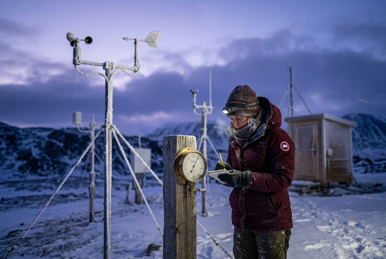
1. Opening Scene: The Sudden Descent of the Iron Curtain

Step onto the crest of an exposed chalk down in southern England or a granite ridge overlooking the Hudson Valley in late January, and the atmosphere often tells its grandest tales through an unsettling stillness. For three weeks, your winters have been defined by an incessant, sodden maritime regime: mild, blustery south-westerlies rolling off the ocean, bringing temperatures hovering stubbornly near 11°C (52°F), muddy pastures, and grey stratocumulus clouds skittering overhead. You have not worn your heavy woollen coat all month.

Then, across forty-eight hours, the invisible architecture of the northern hemisphere shifts.

The first physical sensation is not cold, but weight. Your ears pop subtly as you ascend the ridge; the pocket aneroid barometer in your rucksack has ceased its restless bouncing and climbed relentlessly past 1020 hectopascals, then 1030, finally stabilizing at an imposing 1042 hPa. The damp, humid scent of decaying leaves and wet loam vanishes, purged by an air mass so desiccated that your lips immediately chap.

=========================================================================
SYNOPTIC BAROMETRIC SHIFT: POSITIVE VS NEGATIVE ARCTIC OSCILLATION (AO)
=========================================================================
      POSITIVE AO PHASE (+)                  NEGATIVE AO PHASE (-)
   [Frigid Air Trapped at Pole]          [Frigid Air Discharged South]

970 hPa (Deep Low)                    1045 hPa (Blocking High)
             .---.                                   .---.
            / Polar\                                / Polar\
           (  Cap   )                              (  Cap   )
            \      /                                \      /
             '---'                                   '---'
               ^                                       |
    ============== Zonal Jet =============             | Arctic Outbreak
         --->  FAST WESTERLIES --->                    v
    ======================================     ~~~~~ Buckling Jet ~~~~~
                                              /      (Deep Troughs)    \
          1025 hPa (Subtropical High)        /                          \
             Mid-Latitudes                     1010 hPa (Mid-Latitudes)
=========================================================================

Look upward. The low, ragged cloud base dissolves into a crystalline, pale-cobalt sky. There is no haze, no softening of the horizon. As twilight approaches, the wind—which had died to a breathless lull—resurrects itself from an entirely new quarter. It does not arrive from the west. It blows out of the east-northeast, a thin, laminar draught that cuts through fleece and denim with scalpel-like precision.

By nightfall, the temperature is falling at a rate of two degrees every hour. Frost does not merely coat the grass blades; it forms thick, dagger-like rime on fence posts, telegraph wires, and dry stone walls. By morning, you are enveloped in a deep, subzero continental freeze that will not yield for a fortnight. Half a world away, meteorologists monitoring hemispheric satellite loops and stratospheric soundings nod in unison: the polar cap has tipped its contents into the mid-latitudes. The Arctic Oscillation has crashed into its negative phase.

2. What Is Actually Happening? Plain English First

To understand why a winter landscape can pivot so violently from mild dampness to arctic paralysis, think of the Northern Hemisphere’s atmosphere not as a chaotic soup, but as a giant, fluid spinning top balanced over the North Pole.

The atmosphere behaves like a layered, circulating fluid over a rotating sphere. At the equator, intense solar heating causes warm air to expand and rise; at the North Pole, months of total darkness and perpetual radiation to outer space chill the air into a dense, heavy, shrinking dome. This fundamental temperature contrast creates a steep planetary pressure slope from south to north.

Because the Earth rotates beneath this air mass from west to east, the air flowing toward the pole is deflected by the Coriolis force into a roaring, circumpolar river of wind: the polar jet stream.

=========================================================================
HEMISPHERIC JET STREAM TOPOLOGY IN POLAR PROJECTION
=========================================================================

POSITIVE PHASE (+AO)                     NEGATIVE PHASE (-AO)
      ----------------------                   ----------------------
         TIGHT POLAR LASSO                     WOBBLING, LOOPING WAVE

N                                       N
             .-------.                               . - ~ ~ - .
          .-'   LOW   '-.                        .-'    HIGH     '-.
        .'    (Polar)    '.                    .'      (Polar)      '.
       /                   \                  /   ^             |     \
      |   ===> JET ===>     |                |    |             |      |
      |   (Fast & Zonal)    |                | Ridge (Warm)    Trough  |
       \                   /                  \   |             | (Cold)\
        '.               .'                    '. |             v     .'
          '-.  HIGH   .-'                        '-.    LOW      .-'
             '-------'                               ' - ~ ~ - '
          (Mid-Latitudes)                          (Mid-Latitudes)
=========================================================================

Atmospheric scientists refer to the grand, pulsating rhythm of this system as the Arctic Oscillation (AO), or more formally in academic literature, the Northern Annular Mode (NAM). It is a hemispheric-scale seesaw of atmospheric mass operating between the high Arctic (north of 60°N) and the mid-latitude belt of Europe, Asia, and North America (around 40°N–50°N).

The Positive Phase (+AO): The Tight Atmospheric Lasso

When the Arctic Oscillation is in its positive phase, sea-level pressure over the polar cap plunges far below its long-term average, while pressure across the mid-latitudes rises.

Think of this state as an exceptionally tight, rapidly spinning ice skater. The pressure difference between the high Arctic and the temperate zones is vast and steep. This steep gradient spins up a fierce, locked ribbon of westerly winds encircling the Arctic like a giant atmospheric lasso. Frigid, subzero air masses are corralled tightly within the Arctic basin.

For residents in London, New York, Frankfurt, or Seattle, a positive AO locks the weather into a relentless zonal pattern: * Pacific and Atlantic storm tracks steer mild ocean air across continents. * Freezing outbreaks are suppressed. * Winters remain damp, stormy, and largely snow-free.

The Negative Phase (-AO): The Buckling Fence and Polar Outbreak

When the Arctic Oscillation flips into its negative phase, the seesaw tilts the other way. High pressure builds explosively over the polar cap—most famously manifesting as colossal, stubborn anticyclones over Greenland, northern Canada, or the Arctic Ocean. Simultaneously, pressure over the mid-latitudes drops.

Returning to our spinning top analogy, as the top slows down, it begins to wobble violently. The pressure gradient between the pole and the mid-latitudes slackens or reverses entirely. Deprived of the sharp pressure drop that maintains its high-speed zonal circuit, the circumpolar jet stream decelerates and destabilizes.

Instead of running straight from west to east, the jet stream buckles into gigantic, wandering S-shaped curves known as planetary Rossby waves: 1. Amplified Ridges: Massive domes of warm, subtropical air surge far north into Alaska and Greenland. 2. Deep Troughs: Giant, southward-plunging loops carve out channels for dense, bone-chilling Arctic air to drain south into Chicago, Madrid, Beijing, or southern England.

The polar fence has collapsed. The frigid reservoir built up over months of polar darkness spills out across the continents, initiating prolonged subzero spells, blizzard conditions, and severe agricultural frosts.

The phenomenon exhibits what dynamic meteorologists call an equivalent barotropic structure: the pressure anomalies seen at sea level are not shallow surface features, but vertically aligned pillars of anomalous air mass that extend from the Earth's surface through the troposphere and deep into the stratosphere.

When a Sudden Stratospheric Warming (SSW) event occurs 30 kilometres above the North Pole, it shatters the stratospheric polar vortex; over the subsequent two to four weeks, those anomalies propagate downward to the surface, locking the AO into a severe negative phase that can freeze continents for over a month.

3. The Science: Mathematical Grounding & Dynamic Proofs

For those who wish to peer into the thermodynamic and fluid-mechanical engine room, the Arctic Oscillation is not a mere descriptive label; it is a precisely quantifiable mode of variability governed by fundamental physical equations.

The Arctic Oscillation Index: Principal Component Analysis

The mathematical state of the Arctic Oscillation at time $t$, denoted as $I_{\text{AO}}(t)$, is officially defined by meteorological centers like the NOAA Climate Prediction Center (CPC) and the European Centre for Medium-Range Weather Forecasts (ECMWF) using the leading Empirical Orthogonal Function (EOF-1) of monthly or daily mean sea-level pressure (SLP) or geopotential height anomalies ($Z'$) north of 20°N:

$$I_{\text{AO}}(t) = \frac{\sum_{i=1}^{M} w_i \cdot Z'i(t) \cdot e{1,i}}{\sigma_{\text{AO}}}$$

Where: * $Z'i(t) = Z_i(t) - \overline{Z}_i$ is the geopotential height anomaly at spatial grid point $i$. * $w_i = \sqrt{\cos(\phi_i)}$ represents latitude-dependent grid weighting accounting for the convergence of meridians toward the pole. * $e{1,i}$ is the first spatial eigenvector (EOF-1) representing the annular dipolar seesaw. * $\sigma_{\text{AO}}$ is the standard deviation used to normalize the index to unit variance ($\mu = 0, \sigma = 1$).

When $I_{\text{AO}} > +1.5$, the polar vortex is exceptionally contracted and intense; when $I_{\text{AO}} < -1.5$, the hemisphere enters a major blocking and cold-wave regime.

Equation 1: Geostrophic Wind Balance and Jet Stream Acceleration

To quantify how polar pressure variations directly modulate the speed of the winds aloft, we invoke the geostrophic wind balance ($u_g$). On synoptic scales, horizontal air motion represents an equilibrium between the horizontal Pressure Gradient Force (PGF) pushing air toward low pressure, and the Coriolis force deflecting air to the right in the Northern Hemisphere.

In Cartesian coordinates on a local tangent plane ($x$ pointing east, $y$ pointing north):

$$u_g = -\frac{1}{f \rho} \left( \frac{\partial P}{\partial y} \right)_z = -\frac{g}{f} \left( \frac{\partial Z}{\partial y} \right)_p$$

Where: * $u_g$ is the zonal (east-west) geostrophic wind component ($\text{m/s}$). Positive values denote westerly winds (blowing from west to east); negative values denote easterly winds. * $f = 2\Omega \sin\phi$ is the Coriolis parameter ($\text{s}^{-1}$), where $\Omega = 7.2921 \times 10^{-5}\text{ rad/s}$ is the Earth's angular rotation rate and $\phi$ is the latitude. * $\rho$ is the atmospheric air density ($\text{kg/m}^3$). * $g = 9.80665\text{ m/s}^2$ is gravitational acceleration. * $\left( \frac{\partial P}{\partial y} \right)_z$ is the meridional pressure gradient across lines of latitude at constant geometric height $z$. * $\left( \frac{\partial Z}{\partial y} \right)_p$ is the slope of the geopotential height surface on a constant isobaric pressure level (such as 500 hPa).

Worked Synoptic Proof: Positive vs. Negative AO Wind Response

Let us evaluate the zonal wind at mid-latitudes ($\phi = 55^\circ\text{N}$) spanning the 2,220-kilometre distance ($\Delta y$) between $45^\circ\text{N}$ (Central Europe / Northern US) and $65^\circ\text{N}$ (Iceland / Subpolar Basin).

First, calculate the local Coriolis parameter at $\phi = 55^\circ\text{N}$:

$$f = 2 \cdot (7.2921 \times 10^{-5}\text{ s}^{-1}) \cdot \sin(55^\circ) = 1.45842 \times 10^{-4} \cdot 0.81915 \approx 1.1947 \times 10^{-4}\text{ s}^{-1}$$

Taking a standard surface air density $\rho \approx 1.25\text{ kg/m}^3$, the denominator product is:

$$f \cdot \rho = (1.1947 \times 10^{-4}\text{ s}^{-1}) \cdot (1.25\text{ kg/m}^3) \approx 1.4934 \times 10^{-4}\text{ kg}/(\text{m}^3\cdot\text{s})$$

The meridional distance across $20^\circ$ of latitude is:

$$\Delta y = 20^\circ \times 111.13\text{ km/deg} = 2.2226 \times 10^6\text{ m}$$

Case A: Strong Positive AO Phase (+AO)

A deep subpolar low ($P_{65^\circ\text{N}} = 980\text{ hPa} = 98,000\text{ Pa}$) confronts a strong mid-latitude Azores-Bermuda high ($P_{45^\circ\text{N}} = 1020\text{ hPa} = 102,000\text{ Pa}$).

Calculate the pressure difference: $$\Delta P = P_{65^\circ\text{N}} - P_{45^\circ\text{N}} = 98,000\text{ Pa} - 102,000\text{ Pa} = -4,000\text{ Pa}$$
Compute the horizontal pressure gradient: $$\frac{\partial P}{\partial y} \approx \frac{\Delta P}{\Delta y} = \frac{-4,000\text{ Pa}}{2.2226 \times 10^6\text{ m}} \approx -1.7997 \times 10^{-3}\text{ Pa/m}$$
Compute the resulting zonal geostrophic wind: $$u_g = -\frac{1}{1.4934 \times 10^{-4}} \cdot (-1.7997 \times 10^{-3}) = +12.05\text{ m/s} \approx 43.4\text{ km/h}\text{ (23.4 knots)}$$

💡 NOTE

Positive Phase Dynamics Result: The atmosphere generates a strong, stable +12.05 m/s westerly gale. This fierce west-to-east flow fences the polar air north of the Arctic circle and floods mid-latitude continents with maritime warmth.

Case B: Severe Negative AO Phase (-AO)

A massive Greenland/Arctic blocking anticyclone builds to $P_{65^\circ\text{N}} = 1036\text{ hPa} = 103,600\text{ Pa}$, while the mid-latitude pressure drops to $P_{45^\circ\text{N}} = 1012\text{ hPa} = 101,200\text{ Pa}$.

Calculate the pressure difference: $$\Delta P = P_{65^\circ\text{N}} - P_{45^\circ\text{N}} = 103,600\text{ Pa} - 101,200\text{ Pa} = +2,400\text{ Pa}$$
Compute the horizontal pressure gradient: $$\frac{\partial P}{\partial y} \approx \frac{+2,400\text{ Pa}}{2.2226 \times 10^6\text{ m}} \approx +1.0798 \times 10^{-3}\text{ Pa/m}$$
Compute the resulting zonal geostrophic wind: $$u_g = -\frac{1}{1.4934 \times 10^{-4}} \cdot (+1.0798 \times 10^{-3}) = -7.23\text{ m/s} \approx -26.0\text{ km/h}\text{ (-14.1 knots)}$$

⭐ IMPORTANT

Negative Phase Dynamics Result: The zonal westerly jet does not merely weaken—it completely reverses into a -7.23 m/s easterly flow. This complete breakdown of the zonal barrier permits cold continental air to surge directly westward and southward into temperate maritime zones.

Equation 2: The Thermal Wind Relation and Rossby Wave Buckling

Why does the jet stream buckle into wandering loops when the zonal wind slows? The answer lies in the thermal wind equation, which links vertical wind shear directly to horizontal temperature gradients:

$$\frac{\partial u_g}{\partial \ln p} = \frac{R_d}{f} \left( \frac{\partial T}{\partial y} \right)_p$$

Where $R_d = 287.05\text{ J/(kg}\cdot\text{K)}$ is the specific gas constant for dry air, and $\left( \frac{\partial T}{\partial y} \right)_p$ is the meridional temperature gradient.

According to Rossby wave dispersion theory, the phase speed $c$ of planetary waves in the mid-troposphere is given by:

$$c = \bar{u} - \frac{\beta}{K^2}$$

Where $\bar{u}$ is the mean zonal wind speed, $\beta = \frac{\partial f}{\partial y} = \frac{2\Omega \cos\phi}{a}$ is the Rossby parameter (gradient of the Coriolis force with planetary radius $a$), and $K^2 = k_x^2 + k_y^2$ is the total horizontal wavenumber squared.

When the Arctic Oscillation collapses into a deep negative state, the mean zonal wind $\bar{u}$ decelerates toward zero ($\bar{u} \rightarrow 0$). As a mathematical consequence: 1. The phase speed $c$ becomes negative ($c < 0$), causing planetary waves to become retrograde (moving east-to-west) or entirely stationary ($c \approx 0$). 2. The wave amplitude grows explosively through non-linear baroclinic energy conversion, bending the jet stream into deep, high-amplitude meridional troughs that remain locked over continents for weeks.

4. Practical Outdoor Guidance: Reading the Sky and Instruments

You do not need access to a supercomputing cluster at the UK Met Office or the World Meteorological Organization to recognize an impending phase transition of the Arctic Oscillation. The atmosphere leaves unmistakable signatures across your local sky, barometer, and wind vane.

=========================================================================
SYNOPTIC CHECKLIST FOR THE OUTDOOR OBSERVER: -AO ARRIVAL
=========================================================================
  INSTRUMENT / SENSOR   | TRANSITION SIGNATURE      | SYNOPTIC MEANING
------------------------+---------------------------+--------------------
  Aneroid Barometer     | Steady rise to >1035 hPa  | Polar block forming
  Digital Barograph     | Convex, plateauing trace  | Cold air dome seating
  Wind Vane             | Clockwise veer (SW -> NE) | Continental advection
  Psychrometer (RH)     | Dew point plunges <-10°C  | Arctic air displacement
  All-Sky View          | Optically clear, halos    | Ice crystal suspension
=========================================================================

1. What to Look for in the Sky

The High-Altitude Messenger (Cirrus Uncinus from the "Wrong" Direction): In normal mid-latitude winter weather, cirrus clouds travel rapidly from west to east. When an Arctic blocking high establishes itself to your north, look for thin, hooked cirrus plumes (mare’s tails) arriving from the north-northeast or east. This confirms that the entire tropospheric steering flow has reversed.
The Optical Halo Phenomena: Arctic air masses descending from the polar cap are extraordinarily dry at the surface but carry sub-microscopic, hexagonal ice crystals in suspension throughout the boundary layer (diamond dust). Watch for sharp 22° solar halos, parhelia (sun dogs), and vertical light pillars extending above streetlights at dusk.
The "Barometric Lid" Inversion: Under the descending branch of a polar anticyclone, intense subsidence warms the upper air, creating an impenetrable thermal inversion. Smoke from woodstoves and chimneys will flatten horizontally like a tabletop at 100 metres altitude, unable to penetrate the dense, cold air layer hugging the frozen turf.

2. Instrument Readings to Track

The Barometer: Watch for the "Greenland/Scandi Block" pattern. If your barometer rises steadily during an active cold front and stabilizes well above 1035 hPa without the arrival of mild weather, you are under the influence of an Arctic-origin anticyclone.
The Psychrometer (Dew Point Depression): Track the dew point rather than air temperature alone. Maritime polar air may bring temperatures of 2°C with a dew point of 0°C. True Arctic air from a negative AO outbreak will cause the dew point to crash to -12°C or lower even while daytime surface temperatures remain near freezing. This vast dew point depression indicates a continental air mass with origins in polar permafrost basins.
The Wind Vane: A classic negative AO transition features a slow, clockwise veering of the wind: starting at south-west, sweeping through north-west, settling into north-east, and locking there with persistent gusts.

3. Field Rules for Observers

For Hikers and Climbers: Be aware that the dense, dry air of a negative AO polar outbreak increases atmospheric drag and accelerates convective heat loss. A 20 km/h wind in -10°C Arctic air strips body heat three times faster than in wet maritime air of the same temperature due to extreme vapor pressure deficits. Check ice safety, as small lakes can freeze solid within 72 hours under severe radiative cooling.
For Gardeners and Farmers: The transition to a -AO regime brings devastating radiative frosts. When the wind drops under a 1040 hPa Arctic dome on a cloudless night, the surface temperature can plunge 8°C below the official shelter (2-metre) temperature due to intense terrestrial blackbody radiation escaping directly to space. Apply thick organic mulches and fleece wraps before the wind veers east.
For Mariners and Coastal Observers: When frigid continental air ($T_{\text{air}} < -10^\circ\text{C}$) streams over relatively warm coastal waters ($T_{\text{water}} \approx +8^\circ\text{C}$), the extreme air-sea temperature differential creates steam fog (Arctic sea smoke). Watch for violent localized convective snow squalls—the maritime consequence of a buckling polar jet.

5. Today's Meteorological Rule of Thumb

✨ TIP

The Polar Seesaw Principle: When the winter barometer climbs high but the wind locks stubbornly into the north-east, the polar fence has broken. Expect the freeze to last weeks, not days.