Quantum Cramér-Rao Bound: Deriving Ultimate Parameter Estimation Limits and Symmetric Logarithmic Derivatives in Quantum Metrology
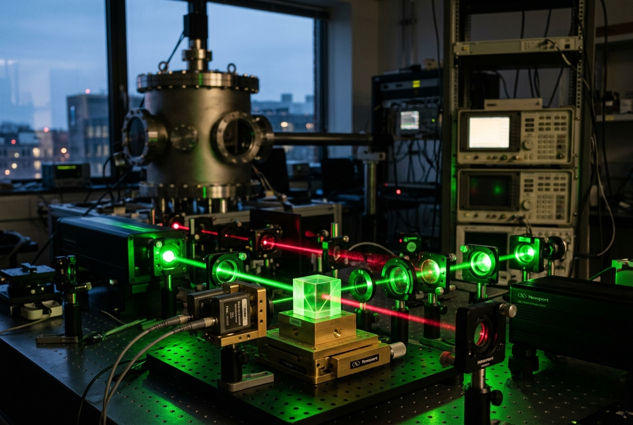
Every measurement ever performed is a conversation with noise. When an astronomer measures the subtle redshift of distant starlight, when an engineer measures the flight time of a laser pulse inside a GPS satellite, or when a magnetic resonance scanner maps water molecules in living human tissue, the goal is identical: to infer the value of an unknown physical quantity from a finite collection of imperfect signals.
For nearly a century, classical statistics dictated the ultimate boundary of this inference. If you repeated an experiment $N$ times, your statistical uncertainty could shrink, at best, in proportion to one over the square root of $N$. This rule—known across the sciences as the shot-noise or standard quantum limit—felt as immutable as the laws of thermodynamics.
Yet deep within the architecture of quantum mechanics lies an extraordinary loophole. In 1967, the physicist Carl W. Helstrom showed that when information is imprinted not onto classical voltages or counting rates, but directly into the fragile geometry of entangled quantum states, the rules of measurement change. The ultimate attainable precision is governed not by classical noise distributions, but by an absolute physical boundary: the Quantum Cramér-Rao Bound (QCRB).
By leveraging quantum entanglement and squeezing, quantum sensors can fundamentally surpass classical bounds, achieving measurement sensitivities scaling directly with $1/N$—the legendary Heisenberg limit. Today, this mathematical framework is no longer an abstract curiosity of quantum information theory. It orchestrates the operation of our planet's most sensitive instruments, from the laser arms of the LIGO Scientific Collaboration detecting the whisper of colliding black holes across the cosmos, to atomic clocks synchronizing the modern financial grid.
1. Foundations of Parameter Estimation: The Classical-to-Quantum Divide
To understand what makes the quantum bound so radical, we must first examine the classical foundation upon which it is built: the Cramér-Rao bound, established independently by Harald Cramér and C. R. Rao in the mid-1940s.
In classical statistical estimation, an experimenter seeks to determine an unknown continuous parameter $\theta$ (such as temperature, voltage, or time delay) by drawing random sample data $x$ from a probability distribution $p(x|\theta)$. Any unbiased estimator $\hat{\theta}(x)$—a mathematical rule that maps raw data to an estimate of $\theta$ without systematic offset—has an inherent variance. The classical Cramér-Rao inequality proves that this variance is bounded from below by the reciprocal of the Classical Fisher Information (CFI), denoted $I(\theta)$:
$$\mathrm{Var}(\hat{\theta}) \ge \frac{1}{M \, I(\theta)}$$
where $M$ is the number of independent measurement runs. The classical Fisher information measures how sensitively the log-likelihood of observing data $x$ changes in response to an infinitesimal shift in the true parameter:
$$I(\theta) = \mathbb{E}\left[ \left( \frac{\partial \ln p(x|\theta)}{\partial \theta} \right)^2 \right] = \int dx \, p(x|\theta) \left( \frac{\partial \ln p(x|\theta)}{\partial \theta} \right)^2$$
If a tiny change in $\theta$ dramatically reshapes the probability distribution $p(x|\theta)$, $I(\theta)$ is large, the statistical landscape possesses steep gradients, and the parameter can be estimated with high precision. Conversely, if $p(x|\theta)$ barely budges when $\theta$ changes, $I(\theta)$ is near zero, and distinguishing neighboring parameter values becomes impossible.
The Quantum Problem
In quantum mechanics, this classical paradigm breaks down because the parameter $\theta$ is rarely a direct physical observable represented by a self-adjoint operator. Instead, $\theta$ is encoded into the state of a quantum system through physical dynamics—either via unitary evolution governed by a Hamiltonian $H$, where the initial state evolves as $\rho(\theta) = e^{-i H \theta / \hbar} \rho_0 e^{i H \theta / \hbar}$, or via open, dissipative dynamics modeled by a Lindblad master equation.
Consequently, there is no predetermined classical probability distribution $p(x|\theta)$. The probability distribution appears only after the experimentalist chooses a quantum measurement, mathematically represented by a Positive Operator-Valued Measure (POVM)—a set of positive semi-definite operators ${\Pi_x}$ that sum to the identity operator, $\sum_x \Pi_x = \mathbb{I}$. According to Born's rule, the probability of obtaining outcome $x$ given parameter $\theta$ is:
$$p(x|\theta) = \mathrm{Tr}\left( \rho(\theta) \Pi_x \right)$$
Every chosen measurement strategy ${\Pi_x}$ yields a distinct classical probability distribution, and therefore a distinct classical Fisher information $I_{{\Pi_x}}(\theta)$. This leads to a fundamental question at the core of quantum metrology: What is the absolute maximum Fisher information that can be extracted from a parameterized quantum state $\rho(\theta)$ over all possible quantum measurements allowed by physics?
2. The Symmetric Logarithmic Derivative: The Quantum Score Operator
In classical statistics, the quantity $\partial_\theta \ln p(x|\theta) = \frac{1}{p(x|\theta)} \frac{\partial p(x|\theta)}{\partial \theta}$ is known as the score function. When we attempt to construct a quantum analog of the score function by differentiating the density operator $\rho(\theta)$, we run into a major obstacle: the non-commutative nature of quantum operators. Because $\rho(\theta)$ does not in general commute with its derivative $\frac{\partial \rho(\theta)}{\partial \theta}$, we cannot simply divide matrices or write a straightforward operator logarithm derivative.
To preserve the hermiticity and symmetry of the resulting observable, Helstrom introduced the Symmetric Logarithmic Derivative (SLD) operator, denoted $L_\theta$. The SLD is defined implicitly as the self-adjoint operator that satisfies the matrix Lyapunov equation:
$$\frac{\partial \rho(\theta)}{\partial \theta} = \frac{1}{2} \left( \rho(\theta) L_\theta + L_\theta \rho(\theta) \right)$$
This symmetrized anticommutator structure ensures that $L_\theta = L_\theta^\dagger$ is a valid quantum observable representing the optimal quantum score.
Spectral Resolution of the SLD
To solve for $L_\theta$ explicitly, we express the density operator $\rho(\theta)$ in its instantaneous spectral decomposition:
$$\rho(\theta) = \sum_{j} p_j |j\rangle \langle j|$$
where ${p_j}$ are the non-negative eigenvalues representing the state populations ($\sum_j p_j = 1$), and ${|j\rangle}$ forms an orthonormal basis of eigenvectors depending on $\theta$.
Differentiating $\rho(\theta)$ and projecting the defining SLD relation into this eigenbasis yields the matrix elements of $L_\theta$:
$$\langle j | \frac{\partial \rho}{\partial \theta} | k \rangle = \frac{1}{2} \langle j | (\rho L_\theta + L_\theta \rho) | k \rangle = \frac{p_j + p_k}{2} \langle j | L_\theta | k \rangle$$
For any pair of states where $p_j + p_k > 0$, we can invert this expression directly. The matrix elements of the SLD operator are given by:
$$\langle j | L_\theta | k \rangle = \frac{2}{p_j + p_k} \langle j | \frac{\partial \rho(\theta)}{\partial \theta} | k \rangle$$
For indices where $p_j + p_k = 0$, the corresponding matrix elements do not contribute to physical expectation values and can be set to zero.
The SLD operator $L_\theta$ captures two distinct physical effects simultaneously: 1. Population shifts: The diagonal elements $\langle j | L_\theta | j \rangle = \frac{1}{p_j} \frac{\partial p_j}{\partial \theta}$ represent classical probability redistribution among eigenstates. 2. Coherence rotations: The off-diagonal elements $\langle j | L_\theta | k \rangle$ ($j \neq k$) reflect the rotation of the quantum state's eigenbasis in Hilbert space, driven by quantum coherences.
3. The Quantum Fisher Information and the Proof of the QCRB
With the SLD established, we can define the Quantum Fisher Information (QFI), denoted $F_Q(\theta)$, as the expectation value of the squared SLD operator:
$$F_Q(\theta) = \mathrm{Tr}\left( \rho(\theta) L_\theta^2 \right) = \frac{1}{2} \mathrm{Tr}\left( \frac{\partial \rho(\theta)}{\partial \theta} L_\theta \right)$$
Substituting the spectral resolution into this trace yields the canonical analytical formula for the QFI of an arbitrary mixed state:
$$F_Q(\theta) = \sum_{j} \frac{(\partial_\theta p_j)^2}{p_j} + 2 \sum_{j \neq k} \frac{(p_j - p_k)^2}{p_j + p_k} |\langle j | \partial_\theta k \rangle|^2$$
where the first sum is purely classical (Fisher information from eigenvalue dynamics), and the second sum represents purely quantum geometric contributions stemming from the rotation of the eigenspaces.
Derivation of the Quantum Cramér-Rao Inequality
Let ${\Pi_x}$ be an arbitrary POVM measurement performed on the state $\rho(\theta)$, generating measurement outcomes $x$ with probability $p(x|\theta) = \mathrm{Tr}(\rho(\theta) \Pi_x)$. Let $\hat{\theta}(x)$ be any unbiased classical estimator constructed from the measurement record, satisfying $\sum_x p(x|\theta) \hat{\theta}(x) = \theta$.
Differentiating this unbiasedness condition with respect to $\theta$ yields:
$$\sum_x \hat{\theta}(x) \frac{\partial p(x|\theta)}{\partial \theta} = 1$$
Since $\sum_x p(x|\theta) = 1$, we also have $\sum_x \frac{\partial p(x|\theta)}{\partial \theta} = 0$. Subtracting $\theta \sum_x \frac{\partial p(x|\theta)}{\partial \theta} = 0$ allows us to rewrite the derivative as:
$$\sum_x (\hat{\theta}(x) - \theta) \frac{\partial p(x|\theta)}{\partial \theta} = 1$$
Using the definition of the SLD, we substitute $\frac{\partial p(x|\theta)}{\partial \theta} = \mathrm{Tr}\left( \frac{\partial \rho}{\partial \theta} \Pi_x \right) = \mathrm{Re}\left[ \mathrm{Tr}\left( \rho L_\theta \Pi_x \right) \right]$:
$$1 = \sum_x (\hat{\theta}(x) - \theta) \mathrm{Re}\left[ \mathrm{Tr}\left( \rho L_\theta \Pi_x \right) \right] = \mathrm{Re}\left[ \sum_x (\hat{\theta}(x) - \theta) \mathrm{Tr}\left( \sqrt{\rho} L_\theta \sqrt{\Pi_x} \cdot \sqrt{\Pi_x} \sqrt{\rho} \right) \right]$$
Applying the Cauchy-Schwarz inequality for operator inner products $\left|\mathrm{Tr}(A^\dagger B)\right|^2 \le \mathrm{Tr}(A^\dagger A)\mathrm{Tr}(B^\dagger B)$ over the joint sum and trace:
$$1 \le \left( \sum_x (\hat{\theta}(x) - \theta)^2 \mathrm{Tr}(\rho \Pi_x) \right) \left( \sum_x \mathrm{Tr}\left( \sqrt{\rho} L_\theta \Pi_x L_\theta \sqrt{\rho} \right) \right)$$
Observing that $\sum_x (\hat{\theta}(x) - \theta)^2 \mathrm{Tr}(\rho \Pi_x) = \mathrm{Var}(\hat{\theta})$ is the variance of the estimator, and using the completeness relation $\sum_x \Pi_x = \mathbb{I}$ on the second term:
$$\sum_x \mathrm{Tr}\left( \rho L_\theta \Pi_x L_\theta \right) = \mathrm{Tr}\left( \rho L_\theta^2 \right) = F_Q(\theta)$$
Thus, for a single measurement ($M=1$), we obtain the Quantum Cramér-Rao Bound:
$$\mathrm{Var}(\hat{\theta}) \ge \frac{1}{F_Q(\theta)}$$
For $M$ independent, identically distributed measurements on $M$ copies of the state $\rho(\theta)$, the additivity of Fisher information leads immediately to the general form:
$$\mathrm{Var}(\hat{\theta}) \ge \frac{1}{M \, F_Q(\theta)}$$
Saturation of the Bound
The classical Fisher information for any POVM measurement is strictly bounded by the Quantum Fisher Information:
$$I_{{\Pi_x}}(\theta) \le F_Q(\theta)$$
Braunstein and Caves proved in their landmark 1994 paper in Physical Review Letters that for a single parameter $\theta$, the Quantum Cramér-Rao Bound is always saturable.
The equality condition in the Cauchy-Schwarz derivation is achieved when the measurement POVM ${\Pi_x}$ is chosen to be the projective von Neumann measurement onto the eigenbasis of the SLD operator $L_\theta$. In this optimal measurement basis, the classical Fisher information extracted by the detector precisely equals the Quantum Fisher Information: $I_{\mathrm{opt}}(\theta) = F_Q(\theta)$.
4. Geometric Formulation and State Distinguishability
Beyond its role in statistical inference, the Quantum Fisher Information possesses a profound differential-geometric interpretation. In the geometric formulation of quantum mechanics, the set of density operators forms a smooth Riemannian manifold. The QFI defines the natural metric tensor on this manifold of quantum states.
Consider two infinitesimally close quantum states along a trajectory parameterized by $\theta$: the state $\rho(\theta)$ and its neighbor $\rho(\theta + d\theta)$. The distinguishability between these two density matrices is quantified by the Bures distance $d_B(\rho, \sigma)$, defined via the quantum Uhlmann fidelity $\mathcal{F}(\rho, \sigma) = \left( \mathrm{Tr}\sqrt{\sqrt{\rho}\sigma\sqrt{\rho}} \right)^2$:
$$d_B^2(\rho, \sigma) = 2 \left( 1 - \sqrt{\mathcal{F}(\rho, \sigma)} \right)$$
Expanding the Bures distance between neighboring states $\rho(\theta)$ and $\rho(\theta + d\theta)$ via Taylor series yields a direct relationship to the Quantum Fisher Information:
$$d_B^2\left(\rho(\theta), \, \rho(\theta + d\theta)\right) = \frac{1}{4} F_Q(\theta) \, d\theta^2 + \mathcal{O}(d\theta^3)$$
The Quantum Fisher Information is precisely four times the Bures metric tensor component on the quantum state space.
Pure State Geometry and the Fubini-Study Metric
For pure quantum states $\rho(\theta) = |\psi(\theta)\rangle \langle \psi(\theta)|$, the density matrix satisfies $\rho^2 = \rho$, which implies that $\partial_\theta \rho = (\partial_\theta \rho) \rho + \rho (\partial_\theta \rho)$. Consequently, the SLD operator simplifies dramatically to:
$$L_\theta = 2 \frac{\partial \rho(\theta)}{\partial \theta} = 2 \left( |\partial_\theta \psi\rangle \langle \psi| + |\psi\rangle \langle \partial_\theta \psi| \right)$$
Substituting this form into the QFI expression yields the elegant pure-state formula:
$$F_Q(\theta) = 4 \left( \langle \partial_\theta \psi | \partial_\theta \psi \rangle - \left| \langle \psi | \partial_\theta \psi \rangle \right|^2 \right) = 4 \, g_{\theta\theta}^{\mathrm{FS}}$$
where $g_{\theta\theta}^{\mathrm{FS}}$ is the component of the gauge-invariant Fubini-Study metric tensor on the projective Hilbert space of quantum rays, as studied extensively in advanced curricula such as MIT OpenCourseWare Quantum Physics.
If the parameter is imprinted via unitary evolution generated by a time-independent Hamiltonian $\hat{H}$ such that $|\psi(\theta)\rangle = e^{-i \hat{H} \theta / \hbar} |\psi_0\rangle$, the derivative is $|\partial_\theta \psi\rangle = -\frac{i}{\hbar} \hat{H} |\psi(\theta)\rangle$. The Quantum Fisher Information reduces to four times the quantum variance of the generator:
$$F_Q(\theta) = \frac{4}{\hbar^2} \left( \langle \psi_0 | \hat{H}^2 | \psi_0 \rangle - \langle \psi_0 | \hat{H} | \psi_0 \rangle^2 \right) = \frac{4}{\hbar^2} (\Delta \hat{H})^2$$
This reveals that parameter estimation precision is fundamentally governed by the energy fluctuations or generator dispersion of the probe state. Substituting this into the QCRB reproduces the generalized Mandelstam-Tamm time-energy uncertainty relation:
$$\Delta \hat{\theta} \cdot \Delta \hat{H} \ge \frac{\hbar}{2 \sqrt{M}}$$
5. Standard Quantum Limit vs. Heisenberg Limit
The ultimate objective of quantum metrology is to exploit collective quantum phenomena across an ensemble of $N$ physical probes (photons, atoms, or qubits) to maximize the Quantum Fisher Information per particle.
Uncorrelated Probe States: The Standard Quantum Limit
Suppose an experimental probe consists of $N$ identical, non-interacting, uncorrelated particles prepared in a separable product state:
$$\rho_{\mathrm{sep}} = \rho_1 \otimes \rho_2 \otimes \cdots \otimes \rho_N$$
If each particle independently undergoes a phase shift generated by the local Hamiltonian $h^{(k)}$, the global generator is the linear sum $\hat{H} = \sum_{k=1}^N h^{(k)}$.
Because there are no cross-correlations between distinct particles ($\langle h^{(j)} h^{(k)} \rangle = \langle h^{(j)} \rangle \langle h^{(k)} \rangle$ for $j \neq k$), the total variance is strictly additive:
$$(\Delta \hat{H}){\mathrm{sep}}^2 = \sum{k=1}^N (\Delta h^{(k)})^2 = N \, (\Delta h)^2$$
Substituting this variance into the pure-state QFI yields $F_Q(\theta) = 4 N (\Delta h)^2 / \hbar^2$. The resulting minimum parameter uncertainty is bounded by the Standard Quantum Limit (SQL):
$$\Delta \theta_{\mathrm{SQL}} \ge \frac{1}{\sqrt{N F_{Q,1}}} = \frac{\hbar}{2 \sqrt{N} \, \Delta h} \propto \frac{1}{\sqrt{N}}$$
This $\mathcal{O}(1/\sqrt{N})$ scaling represents the classical shot-noise ceiling. Independent coin tosses or uncorrelated photons cannot surpass this limit.
Entangled Probe States: Reaching the Heisenberg Limit
Now consider an ensemble of $N$ two-level systems (qubits) prepared in a maximally entangled Greenberger-Horne-Zeilinger (GHZ) state:
$$|\mathrm{GHZ}\rangle = \frac{1}{\sqrt{2}} \left( |0\rangle^{\otimes N} + |1\rangle^{\otimes N} \right)$$
Let each qubit accumulate a phase shift $\theta$ via the Pauli generator $\sigma_z / 2$. The total generator is the collective spin operator $\hat{J}z = \frac{1}{2} \sum{k=1}^N \sigma_z^{(k)}$.
Under this evolution, the states transform as $|0\rangle^{\otimes N} \to e^{-i N \theta / 2} |0\rangle^{\otimes N}$ and $|1\rangle^{\otimes N} \to e^{+i N \theta / 2} |1\rangle^{\otimes N}$, yielding the evolved state:
$$|\psi(\theta)\rangle = \frac{1}{\sqrt{2}} \left( e^{-i N \theta / 2} |0\rangle^{\otimes N} + e^{+i N \theta / 2} |1\rangle^{\otimes N} \right)$$
Computing the variance of the collective generator $\hat{J}_z$ on this GHZ state:
$$\langle \mathrm{GHZ} | \hat{J}_z | \mathrm{GHZ} \rangle = 0, \qquad \langle \mathrm{GHZ} | \hat{J}_z^2 | \mathrm{GHZ} \rangle = \frac{1}{2} \left( \frac{N^2}{4} + \frac{N^2}{4} \right) = \frac{N^2}{4}$$
Therefore, $(\Delta \hat{J}_z)^2 = \frac{N^2}{4}$, and the Quantum Fisher Information scales quadratically with particle number:
$$F_Q(\theta) = 4 (\Delta \hat{J}_z)^2 = N^2$$
Substituting this into the Quantum Cramér-Rao Bound reveals the fundamental Heisenberg Limit:
$$\Delta \theta_{\mathrm{HL}} \ge \frac{1}{N}$$
+-------------------------------------------------------------------------------+
|                   SCALING REGIMES IN QUANTUM METROLOGY                         |
|                                                                               |
|   1. Standard Quantum Limit (SQL):    Δθ_SQL  ≥  1 / √N     (Separable)       |
|   2. Heisenberg Limit (HL):          Δθ_HL   ≥  1 / N      (Entangled)       |
|                                                                               |
|   Quantum Advantage Factor:          Gain = √N                                |
+-------------------------------------------------------------------------------+
For $N = 10^6$ particles, the Heisenberg limit offers a potential thousand-fold ($10^3$) enhancement in measurement precision over classical shot noise.
Beyond GHZ states, optical photonic systems utilize NOON states—superpositions of $N$ photons in spatial mode $a$ and zero in mode $b$ with zero in $a$ and $N$ in $b$:
$$|\mathrm{NOON}\rangle = \frac{1}{\sqrt{2}} \left( |N, 0\rangle_{a,b} + |0, N\rangle_{a,b} \right)$$
These states produce an $N$-fold accelerated de Broglie phase oscillation $\propto e^{i N \theta}$, saturating the Heisenberg limit $F_Q = N^2$ for optical phase interferometry. Similarly, spin-squeezed states prepared in atomic ensembles reallocate quantum uncertainty between orthogonal collective spin components, achieving sub-SQL metrological scaling without requiring delicate macroscopic superpositions.
6. Multi-Parameter Estimation and Non-Commutativity
In real-world sensing scenarios, an experimenter often needs to estimate multiple unknown physical parameters simultaneously: $\vec{\theta} = (\theta_1, \theta_2, \dots, \theta_d)^T$. For example, a quantum magnetometer must determine the three spatial vector components of an unknown magnetic field $\vec{B} = (B_x, B_y, B_z)$, or a quantum imaging system must resolve both the transverse location and the separation of two point sources.
When moving to multiple parameters, the scalar QFI becomes a positive semi-definite $d \times d$ Quantum Fisher Information Matrix (QFIM), denoted $\mathbf{F}_Q(\vec{\theta})$, with elements:
$$\left[ \mathbf{F}Q(\vec{\theta}) \right]{jk} = \frac{1}{2} \mathrm{Tr}\left( \rho(\vec{\theta}) { L_{\theta_j}, L_{\theta_k} } \right)$$
where ${A, B} = AB + BA$ is the matrix anticommutator, and $L_{\theta_j}$ is the SLD operator associated with parameter $\theta_j$.
The multi-parameter Quantum Cramér-Rao Bound states that for any positive semi-definite cost weighting matrix $W \ge 0$, the covariance matrix $\mathbf{Cov}(\hat{\vec{\theta}})$ satisfies the matrix inequality:
$$\mathbf{Cov}(\hat{\vec{\theta}}) \ge \frac{1}{M} \mathbf{F}_Q(\vec{\theta})^{-1} \implies \mathrm{Tr}\left( W \mathbf{Cov}(\hat{\vec{\theta}}) \right) \ge \frac{1}{M} \mathrm{Tr}\left( W \mathbf{F}_Q(\vec{\theta})^{-1} \right)$$
The Challenge of Incompatible Observables and the Holevo Bound
Unlike the single-parameter case, the multi-parameter SLD-QCRB is not generally saturable.
The fundamental obstacle is quantum incompatibility: if the optimal SLD operators associated with different parameters do not commute with one another ($[L_{\theta_j}, L_{\theta_k}] \neq 0$), Heisenberg's uncertainty principle prevents the existence of any single physical POVM that simultaneously projects onto the eigenbases of all $L_{\theta_j}$ operators.
The necessary and sufficient condition for the asymptotic multi-parameter SLD-QCRB to be saturable via collective measurements on asymptotic state copies is the weak commutativity condition:
$$\mathrm{Tr}\left( \rho(\vec{\theta}) [L_{\theta_j}, L_{\theta_k}] \right) = 0 \quad \forall j, k$$
When this condition fails, alternative bounds must be used: 1. Right Logarithmic Derivative (RLD) Bound: Defined via $\frac{\partial \rho}{\partial \theta_j} = \rho \mathcal{R}_{\theta_j}$. The RLD metric is complex Hermitian, capturing complementary non-commutative uncertainties. 2. The Holevo Cramér-Rao Bound (HCRB): Developed by Alexander Holevo, this represents the tightest fundamental lower bound on multi-parameter quantum estimation achievable by collective measurements on infinitely many copies of $\rho(\vec{\theta})$. The HCRB minimizes a non-trivial semi-definite program over all possible Hermitian operators satisfying generalized unbiasedness constraints, correctly incorporating the penalty imposed by non-commuting observables.
7. Experimental Implementations and Practical Sensing
The mathematical framework of the Quantum Cramér-Rao Bound provides the benchmark for state-of-the-art quantum technologies, defining performance limits across experimental physics.
+----------------------------------------------------------------------------------------------------+
|                                MODERN QUANTUM METROLOGY PLATFORMS                                  |
+==========================+=============================+===========================================+
| Platform                 | Measured Physical Quantity  | Quantum Resource Utilized                 |
+==========================+=============================+===========================================+
| LIGO / Virgo             | Strain Phase shift (h ~ 10⁻²¹) Frequency-dependent Squeezed Vacuum Light  |
+--------------------------+-----------------------------+-------------------------------------------+
| Optical Lattice Clocks   | Atomic Transition (Δν/ν ~ 10⁻¹⁸) Spin-Squeezed Strontium / Ytterbium Atoms|
+--------------------------+-----------------------------+-------------------------------------------+
| Diamond NV Centers       | Magnetic Field (B ~ pT/√Hz) Multi-spin Coherent Phase Estimation        |
+--------------------------+-----------------------------+-------------------------------------------+
| Optomechanical Cavities  | Force / Displacement (x ~ 10⁻¹⁹ m) Quantum Back-action Evading Measurements|
+--------------------------+-----------------------------+-------------------------------------------+
1. Gravitational-Wave Observatories (LIGO / Virgo)
The Advanced LIGO and Virgo gravitational-wave interferometers detect spacetime ripples that alter their 4-kilometer arm lengths by less than $10^{-19}$ meters—a fraction of the diameter of a proton. The ultimate sensitivity of these laser interferometers is bounded by the Quantum Cramér-Rao Bound applied to continuous-variable bosonic fields.
By injecting frequency-dependent squeezed vacuum states into the dark ports of their beam splitters, as reported in Nature, these observatories suppress quantum phase noise at high frequencies while mitigating quantum radiation pressure noise at low frequencies. This pushes interferometer sensitivity past the standard quantum limit across the audio gravitational-wave band.
2. Trapped-Ion and Optical Lattice Atomic Clocks
Optical lattice atomic clocks at institutions like JILA and NIST manipulate thousands of neutral strontium or ytterbium atoms trapped in optical standing waves. These instruments measure optical clock transition frequencies with systematic uncertainties reaching $10^{-18}$—equivalent to losing less than one second over the entire age of the universe.
The QCRB sets the stability floor for these clocks. By preparing atoms in spin-squeezed states via cavity-mediated collective interactions, atomic clocks surpass the standard quantum limit imposed by single-atom spontaneous emission, substantially reducing the averaging time required for high-precision timekeeping and tests of general relativity.
3. Nitrogen-Vacancy (NV) Centers in Diamond
Nitrogen-vacancy defect centers in diamond host isolated electronic spin triplets ($S=1$) with long coherence times at room temperature. These solid-state atomic probes measure nanoscale magnetic, electric, and thermal fields.
By employing dynamical decoupling sequences and quantum phase estimation algorithms—techniques shared with architectures at IBM Quantum—diamond magnetometers achieve sensitivities below $1\,\mathrm{pT}/\sqrt{\mathrm{Hz}}$. The QCRB provides the theoretical target for these protocols, helping researchers optimize the trade-off between interrogation time and environmental dephasing for nanoscale nuclear magnetic resonance (NMR) imaging of single proteins.
4. Cavity Optomechanics and Force Sensing
Micro- and nano-mechanical resonators coupled to high-finesse optical or microwave cavities serve as ultra-sensitive force detectors, accelerometers, and mass spectrometers.
The QCRB models the fundamental trade-off between measurement imprecision noise and quantum back-action noise (momentum kicks delivered by reflected photons). By implementing back-action evading (BAE) measurement schemes that monitor only a single mechanical quadrature, experimentalists can saturate the QCRB and perform continuous quantum non-demolition force tracking.
8. The Impact: From Foundations to Technology
Why does the Quantum Cramér-Rao Bound matter beyond the laboratory? The answer lies in how precision measurement shapes both technology and fundamental science:
- Navigation in GPS-Denied Environments: Sovereign navigation systems for submarines, aircraft, and spacecraft rely on quantum inertial sensors (accelerometers and gyroscopes). Operating near the Heisenberg limit allows inertial navigation units to maintain drift-free position tracking over months without external satellite signals.
- Medical Diagnostics and Single-Molecule Bio-Imaging: Squeezed light and NV-center magnetometry allow magnetic resonance imaging at the single-cell and single-molecule level. By extracting maximum Fisher information per probe photon, biological samples can be analyzed without thermal damage from high laser powers.
- Probing Fundamental Physics: Whether testing the constancy of fundamental constants ($\alpha$, $G$), searching for ultra-light axionic dark matter candidates, or hunting for deviations from Einstein's equivalence principle, experimental searches are constrained by parameter estimation limits. The QCRB establishes whether an observed null result genuinely rules out a physical theory.
9. Core Takeaway
The Quantum Cramér-Rao Bound establishes that the ultimate precision of any physical measurement is governed not by instrument noise or classical sampling statistics, but by the intrinsic Riemannian geometry of quantum Hilbert space.
By defining the Symmetric Logarithmic Derivative and its associated Quantum Fisher Information, the QCRB reveals that quantum entanglement and squeezing allow measurements to break free from the $1/\sqrt{N}$ Standard Quantum Limit and attain the fundamental $1/N$ Heisenberg Limit. In doing so, the QCRB unites quantum mechanics, information theory, and differential geometry into a single operational framework that defines the boundary of what is knowable in the physical universe.