Equatorial Kelvin Waves & Yanai Wave Dynamics: How Beta-Plane Wave Trapping and Convective Coupling Steer Tropical Weather Systems

1. Opening Scene: The Sudden Breath of the Doldrums

At zero degrees latitude, fifty nautical miles west of Sumatra in the eastern Indian Ocean, the afternoon sea is as flat and vitreous as dark obsidian. The midday sun hangs directly overhead, a searing white disc piercing a canopy of milky haze. The air is suffocatingly dense, hovering at 32°C with a relative humidity near 90 percent. For three consecutive days, your vessel has drifted through the Intertropical Convergence Zone—the maritime doldrums—where the surface wind has collapsed entirely. The water’s surface mirrors the sky so perfectly that the horizon dissolves into an unbroken sheet of slate gray.

Then, without any discernible warning on the local horizon, the atmosphere alters its state.

Your skin registers it first: the oppressive, stagnant stillness breaks as a cool, laminar breeze wafts across the bow from the west, brisk and deliberate, freshening from dead calm to fifteen knots within minutes. The aneroid barometer on the wheelhouse bulkhead, which had been locked in its rhythmic, twice-daily equatorial tidal tick, suddenly drops two full hectopascals below its anticipated baseline.

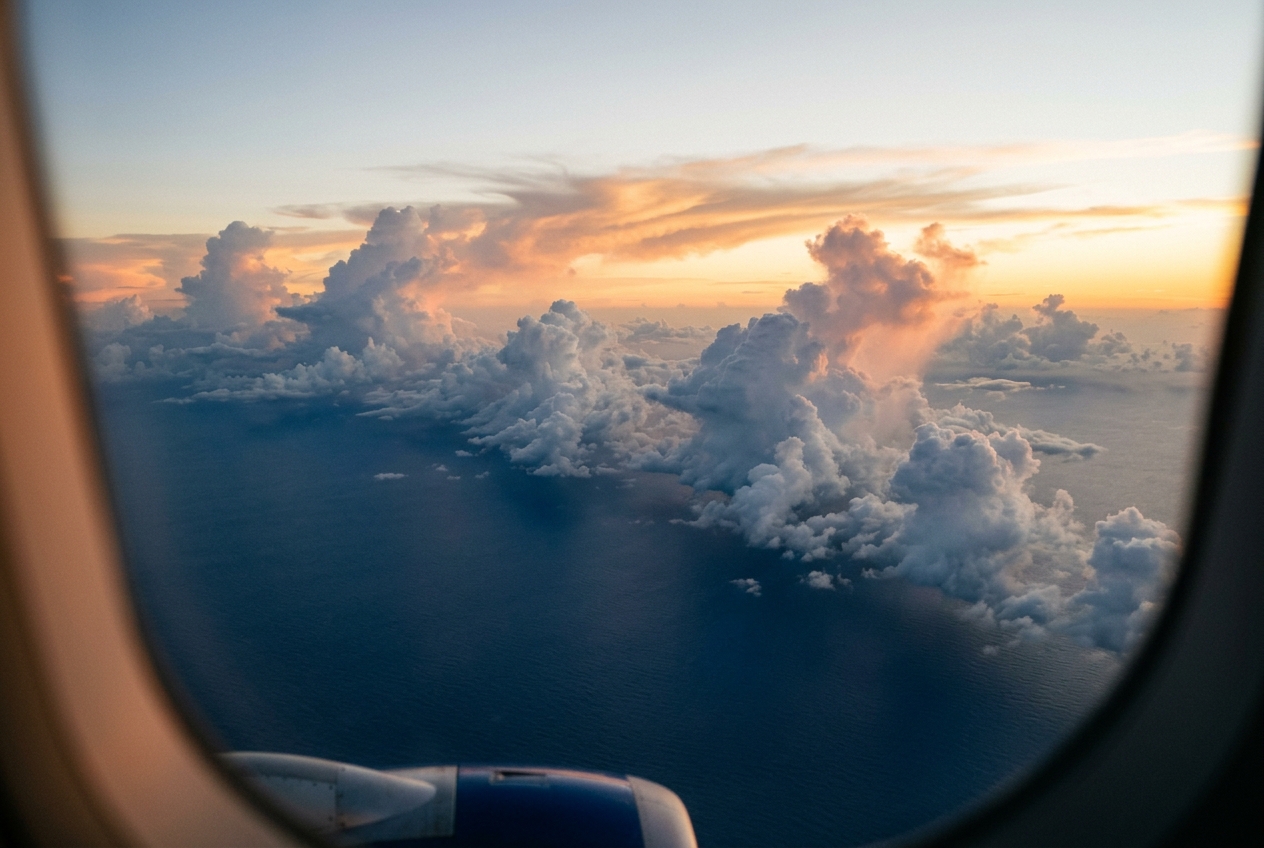
To the west, the pale horizon darkens into a bruised, indigo rampart. A colossal wall of cumulonimbus clouds begins to erupt, mushrooming into the lower stratosphere at tens of meters per second. The air fills with the sharp, metallic scent of ozone and the sudden chill of evaporatively cooled downdrafts. You are not witnessing a random, localized thunderstorm. You are standing in the physical crosshairs of a planetary-scale wave disturbance: an equatorial Kelvin wave, trapped along the Earth's zero-degree parallel, sweeping eastward at thousands of kilometers per day and organizing millions of tons of water vapor into an explosive burst of tropical convection.

2. What's Actually Happening — Plain English First

To understand why the equator is capable of generating such immense, highly organized weather systems, think of our planet’s rotation as a cosmic turnstile that changes direction depending on which hemisphere you occupy.

If you roll a ball across a spinning merry-go-round in the Northern Hemisphere, it curves steadily to your right. In the Southern Hemisphere, the exact same motion curves to your left. This inertial tendency is known as the Coriolis effect. But precisely at the equator, this rotational deflection drops to zero.

Imagine two steep, invisible hills flanking a flat central valley. If you step north of the equator, the planet pushes you back toward the right (southward); if you step south of the equator, the planet pushes you back toward the left (northward). The equator acts as an atmospheric "whispering gallery" or a planetary fiber-optic cable—a dynamic waveguide that traps fluid motions within a narrow tropical corridor roughly a thousand kilometers wide on either side of the zero line.

Within this equatorial channel, the atmosphere dances to two primary rhythms:

1. The Kelvin Wave: Think of the Kelvin wave as an unswerving sprinter. It is an acoustic-gravity wave that travels exclusively from west to east. Because its north-south velocity is strictly zero, the fluid simply sloshes forward and backward along the equator, held in place against the flanking rotational hills.
2. The Yanai Wave (Mixed Rossby-Gravity Wave): Think of the Yanai wave as an acrobatic gymnast. When it ripples across the globe with long wavelengths, it mimics a westward-drifting planetary Rossby wave, dominated by the changing curvature of the Earth. But when its wavelength shortens and its frequency rises, it morphs into an eastward-surging gravity wave. It wiggles serpent-like across the equator, with winds crossing directly from one hemisphere to the other.

When these invisible atmospheric ripples collide with the warm, moisture-laden air of the tropical oceans, they trigger massive boiling towers of rain, modulating global climate patterns across oceans and continents.

3. The Science: Matsuno’s Beta-Plane, Wave Trapping, and Moist Convection

A. The Linearized Shallow Water Equations on an Equatorial $\beta$-Plane

To formalize the dynamics of these trapped equatorial disturbances, we deploy the linearized shallow water equations on an equatorial $\beta$-plane, an enduring theoretical framework pioneered by Matsuno (1966). In the equatorial zone, the Coriolis parameter $f = 2\Omega \sin\phi$ is linearized about latitude $y = 0$ using the approximation $f \approx \beta y$, where:

$$\beta = \left(\frac{df}{dy}\right)_{y=0} = \frac{2\Omega \cos(0)}{a} = \frac{2\Omega}{a} \approx 2.28 \times 10^{-11} \text{ m}^{-1}\text{s}^{-1}$$

Here, $\Omega = 7.292 \times 10^{-5}\text{ rad s}^{-1}$ represents Earth's angular velocity, and $a \approx 6.371 \times 10^6\text{ m}$ is Earth's mean radius.

Let $u$ and $v$ denote the zonal (eastward) and meridional (northward) velocity perturbations, respectively, and let $h$ denote the perturbation of the free-surface height above an undisturbed equivalent depth $H_e$ (or $h_e$). The linearized shallow water system without background mean flow is formulated as:

$$\frac{\partial u}{\partial t} - \beta y v = -g \frac{\partial h}{\partial x}$$

$$\frac{\partial v}{\partial t} + \beta y u = -g \frac{\partial h}{\partial y}$$

$$\frac{\partial h}{\partial t} + H_e \left( \frac{\partial u}{\partial x} + \frac{\partial v}{\partial y} \right) = 0$$

Assuming wave solutions proportional to $e^{i(kx - \omega t)}$, where $k$ is the zonal wavenumber and $\omega$ is the angular frequency, the governing equations transform into a single second-order ordinary differential equation for the meridional velocity structure $\hat{v}(y)$:

$$\frac{d^2 \hat{v}}{dy^2} + \left[ \left( \frac{\omega^2}{c^2} - k^2 - \frac{\beta k}{\omega} \right) - \frac{\beta^2 y^2}{c^2} \right] \hat{v} = 0$$

where $c = \sqrt{g H_e}$ is the intrinsic shallow-water gravity wave speed.

To solve this equation, we define a non-dimensional meridional coordinate $\xi = y / y_0$, where the characteristic equatorial length scale—the equatorial Rossby radius of deformation $y_0$—is defined by:

$$y_0 = \sqrt{\frac{c}{\beta}} = \left(\frac{g H_e}{\beta^2}\right)^{1/4}$$

Under this scaling, the equation takes the canonical form of the quantum harmonic oscillator (Weber's differential equation):

$$\frac{d^2 \hat{v}}{d\xi^2} + \left( \frac{c}{\beta}\left[\frac{\omega^2}{c^2} - k^2 - \frac{\beta k}{\omega}\right] - \xi^2 \right) \hat{v} = 0$$

For the perturbation field to remain bounded as $y \to \pm\infty$ (trapped within the equatorial zone), the eigenvalue condition requires:

$$\frac{c}{\beta}\left( \frac{\omega^2}{c^2} - k^2 - \frac{\beta k}{\omega} \right) = 2n + 1, \quad n = 0, 1, 2, \dots$$

The general solutions are Hermite functions modulated by a Gaussian decay envelope:

$$\hat{v}_n(y) = V_0 H_n\left(\frac{y}{y_0}\right) \exp\left(-\frac{y^2}{2 y_0^2}\right)$$

where $H_n(\xi)$ is the $n$-th Hermite polynomial. The Gaussian term $\exp(-y^2 / 2y_0^2)$ provides mathematical proof that the equatorial $\beta$-plane acts as an intrinsic waveguide: wave energy cannot radiate into the extratropics and remains trapped within a meridional distance $y \sim y_0 \approx 1000\text{--}1500\text{ km}$ of the equator.

B. Proof of the Equatorial Kelvin Wave

The equatorial Kelvin wave is the fundamental boundary-trapped mode corresponding to identically vanishing meridional velocity:

$$v(x,y,t) \equiv 0$$

Setting $v = 0$ collapses the shallow water system into three streamlined equations:

$$\frac{\partial u}{\partial t} = -g \frac{\partial h}{\partial x} \tag{1}$$

$$\beta y u = -g \frac{\partial h}{\partial y} \tag{2}$$

$$\frac{\partial h}{\partial t} + H_e \frac{\partial u}{\partial x} = 0 \tag{3}$$

Equation (2) reveals that the zonal flow is in strict equatorial geostrophic balance: the zonal pressure gradient is balanced solely by the Coriolis acceleration acting on the zonal wind.

Differentiating (1) with respect to $t$ and (3) with respect to $x$, and substituting:

$$\frac{\partial^2 u}{\partial t^2} = -g \frac{\partial}{\partial x}\left( \frac{\partial h}{\partial t} \right) = g H_e \frac{\partial^2 u}{\partial x^2} = c^2 \frac{\partial^2 u}{\partial x^2}$$

This is the classic one-dimensional, non-dispersive wave equation with solutions of the form $u(x,y,t) = U(y) F(x \mp ct)$.

Let us analyze the direction of wave propagation. Differentiating $h = \pm \sqrt{\frac{H_e}{g}} u = \pm \frac{c}{g} u$ and substituting into the geostrophic balance equation (2):

$$\beta y u = -g \left( \pm \frac{c}{g} \frac{dU}{dy} \right) = \mp c \frac{dU}{dy} \implies \frac{1}{U}\frac{dU}{dy} = \mp \frac{\beta y}{c}$$

Integrating with respect to $y$:

$$U(y) = U_0 \exp\left( \mp \frac{\beta y^2}{2c} \right)$$

• For westward propagation ($x + ct$, upper sign $-$): $U(y) = U_0 \exp\left(+\frac{\beta y^2}{2c}\right)$, which grows exponentially toward infinity as $|y| \to \infty$. This solution violates physical boundary conditions and must be rejected.
• For eastward propagation ($x - ct$, lower sign $+$): $U(y) = U_0 \exp\left(-\frac{\beta y^2}{2c}\right)$, which decays symmetrically away from the equator.

Thus, the equatorial Kelvin wave is strictly eastward-propagating and entirely non-dispersive, possessing the dispersion relation:

$$\omega = c k = k \sqrt{g H_e}$$

Its group velocity $c_g$ is identically equal to its phase speed $c_p$:

$$c_g = \frac{\partial \omega}{\partial k} = c = \sqrt{g H_e} = c_p$$

KEY THEORETICAL RESULT: EQUATORIAL KELVIN WAVE PROPERTIES

• Meridional Velocity: $v(x,y,t) = 0$ everywhere.
• Zonal Velocity: $u(x,y,t) = U_0 \exp\left(-\frac{\beta y^2}{2c}\right) \cos(kx - \omega t)$.
• Geopotential Perturbation: $g h(x,y,t) = c U_0 \exp\left(-\frac{\beta y^2}{2c}\right) \cos(kx - \omega t)$.
• Dispersion Law: $\omega = c k \implies c_p = c_g = \sqrt{g H_e}$.

C. Derivation of the Mixed Rossby-Gravity (Yanai) Wave

When $n = 0$, the general dispersion relation yields:

$$\frac{\omega^2}{c^2} - k^2 - \frac{\beta k}{\omega} = \frac{\beta}{c}$$

Multiplying through by $\omega c^2$:

$$\omega^3 - c^2 k^2 \omega - \beta c^2 k - \beta c \omega = 0$$

Factoring this cubic equation yields:

$$(\omega + c k)\left(\omega^2 - c k \omega - \beta c\right) = 0$$

The root $\omega = -c k$ is a spurious mathematical artifact that yields a singular horizontal divergence in the shallow water system. Discarding it leaves the Yanai dispersion relation:

$$\omega^2 - c k \omega - \beta c = 0$$

Solving for $\omega$ using the quadratic formula (selecting the positive physical root $\omega > 0$):

$$\omega(k) = \frac{c k}{2} + \sqrt{\frac{c^2 k^2}{4} + \beta c}$$

The Yanai wave exhibits a remarkable dual dynamical identity across the spectral domain:

1. Short Eastward Wavelengths ($k \gg \sqrt{\beta/c}$): $$\omega \approx \frac{c k}{2} + \frac{c k}{2} = c k$$ The wave behaves as a high-frequency, prograding eastward inertio-gravity wave.
2. Short Westward Wavelengths ($-k \gg \sqrt{\beta/c}$): Expanding the radical via Taylor approximation yields: $$\omega \approx \frac{c k}{2} + \frac{c |k|}{2}\left(1 + \frac{2\beta}{c k^2}\right) = -\frac{c|k|}{2} + \frac{c|k|}{2} - \frac{\beta}{k} = -\frac{\beta}{k}$$ The wave transitions into a low-frequency, retrograding planetary Rossby wave.
3. Zonal Infinite Wavelength ($k = 0$): $$\omega(0) = \sqrt{\beta c}$$ The disturbance manifests as an equatorially trapped, purely meridional inertia-gravity oscillation.

D. Worked Numerical Examples: Dry vs. Moist Dynamics

Let us evaluate the physical scales predicted by these mathematical formulations in both dry dynamic atmospheres and moist convectively coupled regimes.

1. The Dry Free Troposphere (First Internal Baroclinic Mode)

In an idealized dry atmosphere, vertical modal decomposition of the stratification profile yields an equivalent depth corresponding to the first internal baroclinic mode of: $$H_e \approx 250\text{ m}$$

We calculate the dry Kelvin wave speed: $$c_{\text{dry}} = \sqrt{g H_e} = \sqrt{9.81\text{ m s}^{-2} \times 250\text{ m}} = \sqrt{2452.5} \approx 49.5\text{ m s}^{-1} \approx 178\text{ km h}^{-1}$$

The equatorial Rossby radius of deformation is: $$y_{0,\text{dry}} = \sqrt{\frac{c_{\text{dry}}}{\beta}} = \sqrt{\frac{49.5\text{ m s}^{-1}}{2.28 \times 10^{-11}\text{ m}^{-1}\text{s}^{-1}}} = \sqrt{2.17 \times 10^{12}} \approx 1.47 \times 10^6\text{ m} = 1470\text{ km}$$

2. Moist Convectively Coupled Equatorial Kelvin Waves (CCKWs)

When deep tropical cumulonimbus convection couples with the dynamic wave, latent heat release acts as an effective thermal feedback that cancels a large fraction of the dry static stability. According to empirical space-time spectral analyses documented by the National Oceanic and Atmospheric Administration (NOAA) and published in classic studies by Wheeler and Kiladis (1999), the effective equivalent depth collapses to: $$H_e \approx 25\text{ m}$$

Recalculating the phase speed under moist convective coupling: $$c_{\text{moist}} = \sqrt{g H_e} = \sqrt{9.81\text{ m s}^{-2} \times 25\text{ m}} = \sqrt{245.25} \approx 15.66\text{ m s}^{-1} \approx 56.4\text{ km h}^{-1}$$

The trapped equatorial half-width narrows to: $$y_{0,\text{moist}} = \sqrt{\frac{15.66\text{ m s}^{-1}}{2.28 \times 10^{-11}\text{ m}^{-1}\text{s}^{-1}}} \approx 8.28 \times 10^5\text{ m} = 828\text{ km}$$

Moist coupling slows the planetary wave down by a factor of more than three, matching the empirical speed at which tropical cloud clusters march across the Indo-Pacific warm pool.

E. Wheeler-Kiladis Space-Time Spectral Diagrams

How do atmospheric scientists detect these theoretical modes in satellite observations? In their landmark paper, Wheeler and Kiladis (1999) performed two-dimensional Fourier transforms on twice-daily satellite Outgoing Longwave Radiation (OLR) data across longitude and time.

By dividing the raw power spectrum of tropical cloudiness by a smoothed background "red noise" spectrum, they isolated statistically significant peaks in spectral variance.

The resulting Wheeler-Kiladis diagrams confirmed that tropical convection is not stochastic chaos: 1. Convective power aligns along the theoretical Matsuno dispersion curves. 2. The empirical dispersion lines align with equivalent depths between $H_e = 12\text{ m}$ and $H_e = 50\text{ m}$, rather than the dry theoretical values of $200\text{--}300\text{ m}$. 3. This discrepancy provides direct observational evidence that moisture convergence and diabatic heating drastically alter the effective gravity wave speed of the tropical atmosphere.

F. Real-World Case Studies: Weather, Climate, and Cyclogenesis

Equatorial waves are primary engines of global weather variability, tracked daily by the European Centre for Medium-Range Weather Forecasts (ECMWF) and the UK Met Office.

   =============================================================================
   PLANETARY PHENOMENON     DYNAMIC MECHANISM                  WEATHER IMPACT
   =============================================================================
   Convectively Coupled     Eastward surge of low-level        Initiates oceanic
   Kelvin Waves (CCKWs)     westerly wind bursts (WWBs)        downwelling Kelvin waves;
                            at 12-18 m/s; suppresses OLR.      triggers El Niño events.
   -----------------------------------------------------------------------------
   Mixed Rossby-Gravity     Cross-equatorial shear wiggles;    Forms twin cyclones
   (Yanai) Waves            meridional wind oscillations       across the equator in
                            with 4-5 day periods.              Pacific & Indian Oceans.
   -----------------------------------------------------------------------------
   Madden-Julian            CCKWs act as high-frequency        Modulates monsoon breaks,
   Oscillation (MJO)        "building blocks" within the       global atmospheric angular
                            broad MJO envelope.                momentum, and extratropics.
   =============================================================================

1. The Triggering of El Niño via Westerly Wind Bursts

In the western Pacific warm pool, convectively coupled Kelvin waves generate low-level Westerly Wind Bursts (WWBs). These anomalous westerlies produce anomalous surface convergence that downwells the oceanic thermocline. This downwelling creates an oceanic Kelvin wave that surges eastward across the Pacific basin at $2\text{--}3\text{ m s}^{-1}$, flattening the thermocline and initiating major El Niño–Southern Oscillation (ENSO) warm events.

2. Modulating the Madden-Julian Oscillation (MJO)

The Madden-Julian Oscillation (MJO), monitored by the World Meteorological Organization (WMO), is an eastward-moving planetary disturbance with a period of 30–60 days. High-resolution satellite tracking shows that the active convective envelope of the MJO is composed of a hierarchical succession of individual CCKWs. As each Kelvin wave sweeps eastward through the MJO envelope, it triggers localized flare-ups of squall lines and cloud clusters.

3. Yanai Waves and Tropical Cyclogenesis

As Mixed Rossby-Gravity (Yanai) waves propagate westward across the equatorial Pacific and Atlantic, their alternating cross-equatorial wind patterns ($v \neq 0$) generate intense off-equatorial cyclonic vorticity. When a Yanai wave slows near the maritime continent or Central America, its vortical lobes frequently spin off into the Northern and Southern Hemispheres simultaneously, creating "twin tropical cyclones" that flank the equator.

4. Practical Outdoor Guidance

Whether navigating the equatorial shipping lanes, piloting aircraft through the ITCZ, or living along tropical coastlines, equatorial wave passages leave clear physical signatures in the local environment.

What to Look for in the Sky

• The Kelvin Precursor: 24 to 48 hours prior to the arrival of peak convective activity, the high tropical troposphere fills with an extensive sheet of thin, fibrous cirrostratus moving rapidly from west to east. This marks the upper-level divergence plume surging ahead of the surface wave.
• The Squall Front: As the Kelvin wave's surface convergence center arrives, low-level cumulus clouds organize into linear, east-west oriented squall lines, culminating in massive anvil clouds that flatten against the tropical tropopause at 16–18 km altitude.
• The Yanai Wiggle: In a Yanai wave regime, convective clouds alternate their drift direction every 4 to 5 days, shifting from south-southwesterly on Monday to north-northwesterly by Thursday.

Instrument Readings to Monitor

• Aneroid Barometer: The tropical atmosphere is governed by a strict semi-diurnal solar thermal tide, peaking at 10:00 and 22:00 local time and bottoming at 04:00 and 16:00. A persistent deviation of more than $1.5\text{--}2.0\text{ hPa}$ from this harmonic cycle signals the passage of a planetary-scale Kelvin wave trough.
• Wind Vane and Anemometer: In the equatorial belt, winds are normally weak and easterly. A sudden shift to sustained westerly winds exceeding 20 knots ($10\text{ m s}^{-1}$)—a Westerly Wind Burst—is a direct signature of an eastward-passing Kelvin wave.
• Psychrometer/Hygrometer: Look for sharp increases in equivalent potential temperature ($\theta_e$) as warm, moisture-saturated air converges toward the equator from the subtropical trades.

Rule of Thumb for Outdoors

• For Sailors and Mariners: If the barometer drops counter to the daily 10-to-4 tidal rhythm while the wind veers sharply to the west within five degrees of the equator, expect 48 to 72 hours of organized, severe squalls accompanied by an eastward surface current surge.
• For Aviators: Entering the convective envelope of a CCKW means the tropical tropopause will be elevated and turbulent; convective cloud tops will penetrate 1,000–2,000 meters higher than baseline equatorial forecasts.

5. Today's Meteorological Rule of Thumb

THE EQUATORIAL WAVE PRINCIPLE

Because Earth's rotational deflection vanishes at the zero parallel, the equator functions as a natural dynamic waveguide. Kelvin waves march strictly eastward without sloshing north or south, their pace governed by the deep heat release of tropical rain clouds.