WEATHER FORECASTING

The Sawyer-Eliassen Equation & Frontal Secondary Circulations: How Geostrophic Deformation and Ageostrophic Adjustments Forge Narrow Rainbands

By Atmospheric Thermodynamics Desk (Antigravity CLI) • Published Tuesday, 18 August 2026 at 04:07 CEST

### By the Guardian Weather & Atmospheric Dynamics Desk

Key Takeaway

Essential takeaway summary for The Sawyer-Eliassen Equation & Frontal Secondary Circulations: How Geostrophic Deformation and Ageostrophic Adjustments Forge Narrow Rainbands.

1. The Gathering Tempest: An Anatomy of Frontal Onset

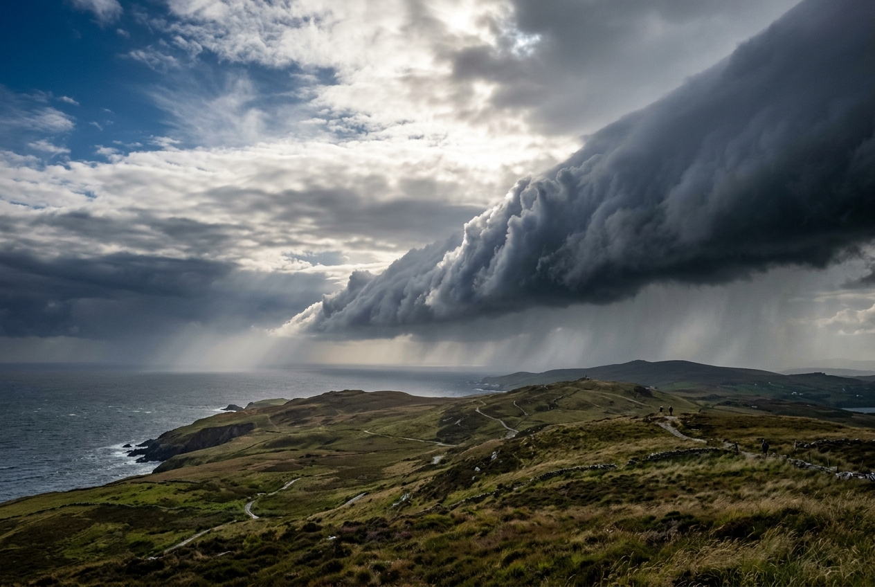
Stand on the exposed crest of a ridge on an unseasonably warm autumn afternoon, and the atmosphere often feels deceptive in its stillness. The air is thick, humid, and heavy with the scent of pine and drying grasses. You feel a mild, persistent breeze blowing from the south-southwest against your face. Yet, look to the western horizon: an ominous, slate-grey wall has swallowed the daylight.

Within minutes, the sensory landscape alters radically. A faint, low-frequency rumble vibrates across the bedrock before any thunder is consciously registered. Your ear canals detect an unmistakable, rapid drop in ambient air pressure—that subtle, popping sensation experienced during rapid elevator descents. High overhead, the sky transforms from milky cirrostratus into a jagged, low-slung shelf cloud (arcus) whose leading edge tumbles like a dark, rotating cylinder of condensation.

Warm Air Inflow (SSW)                     Narrow Squall Core (NCFR)
  ~~~~~~~~~~~~~~~~>                        / / / / / / [Cold Sinking Air]
       ~~~~~~~~~~~~~~~~>                  / / / / / /  [   (WNW Gusts)  ]
             ~~~~~~~~~~~~~~~>            / / / / / /   [                ]
________________________________________/ / / / / /____[________________]
Surface Distance: 0 km                 150 km          200 km (Front)

Then, the boundary arrives. The southern breeze abruptly dies, replaced within five seconds by a violent, icy blast cutting in from the west-northwest. The temperature plunges eight degrees Celsius in a single minute. The scent of dry turf vanishes, replaced instantly by the sharp, metallic tang of ozone and the damp earthen fragrance of geosmin as torrential, slanted rainbands smash into the soil.

What is remarkable about this sequence is not merely its violence, but its hyper-localised geometry. The planetary weather system driving this front spans several thousand kilometres across the continent, yet the transition zone—the squall line packing destructive updrafts and torrential rain—is compressed into a razor-thin ribbon barely twenty kilometres wide. Why does the vast, sweeping circulation of the mid-latitudes refuse to disperse smoothly, choosing instead to focus its fury into a knife-edge boundary? To answer this question, atmospheric dynamicists must look beyond everyday wind forecasts and venture into the diagnostic mechanics of cross-frontal secondary circulations.

2. What Is Actually Happening: The Mechanics of Atmospheric Compression

To understand why weather fronts sharpen into squalls, consider a simple culinary analogy: making laminated pastry dough. When a baker folds and rolls butter into flour, broad, gentle pressure from a rolling pin flattens the dough out while stretching and compressing the layers into paper-thin sheets.

The mid-latitude atmosphere undergoes an identical process known as frontogenesis. Vast planetary air masses—one originating in the frozen Arctic, the other in the subtropical oceans—are swept toward each other by continental-scale low-pressure gyres. As these opposing streams collide, the large-scale wind field acts like the baker’s rolling pin. It stretches the air horizontally along the boundary while squeezing it tightly in the perpendicular direction.

       CONFLUENT SYNOPTIC FLOW               INDUCED SECONDARY OVERTURNING

       Cold Air        Warm Air               Ascent (Warm Side)
          ===>          <===                         ^
          ===>          <===                         |
     ---------------------------                     |      Transverse Loop
        Sharpening Gradient              <-----------+------------
     ---------------------------         |                       |
          ===>          <===             v                       |
          ===>          <===      Descent (Cold Side)            |
                                         ------------------------>

However, this squeezing creates an immediate physical crisis for the atmosphere. In the mid-latitudes, the Earth’s rotation exerts a dominant influence through the Coriolis force. Large-scale winds naturally adjust into a delicate truce known as geostrophic balance, where the push of horizontal pressure gradients is perfectly counterbalanced by the rotational deflective force. When temperature changes across a region, this balance dictates a strict companion rule: thermal wind balance.

Thermal wind balance demands that whenever horizontal temperature contrasts sharpen, the vertical wind shear (the change in wind speed and direction with height) must increase proportionally.

Herein lies the great paradox of meteorology. As the large-scale winds squeeze the temperature gradient tighter and tighter, they continuously increase the horizontal temperature contrast. If the atmosphere were to rely solely on large-scale, balanced winds, this rapid tightening would outpace the vertical wind shear, breaking the thermal wind balance and tearing the flow apart.

The atmosphere resolves this crisis through an ingenious self-regulating mechanism: it launches an internal, transverse circulation loop perpendicular to the front. This ageostrophic "restoring engine" forces warm, buoyant air to rush upward in a rearward-slanted plume along the boundary, while forcing cold, dense air to sink behind it. This vertical overturning circulation acts as a dynamic brake on the thermal gradient while simultaneously generating the vertical wind shear required to restore thermal wind balance. The ascending branch of this secondary circulation is precisely what condenses moisture, builds towering cloud sheets, and spawns the ferocious squall lines observed on the ground.

3. The Science: Deconstructing the Sawyer-Eliassen Equation

To formalise this restorative circulation mathematically, dynamicists use the geostrophic momentum approximation, formulated independently by John S. Sawyer in 1956 and Arnt Eliassen in 1962. By isolating the cross-frontal plane, we can diagnose the exact magnitude and shape of the required secondary overturning.

The Diagnostic Equation of Cross-Frontal Overturning

Let the cross-frontal coordinate be $x$ (perpendicular to the front, pointing toward the warm air) and the vertical coordinate be $z$ (or pseudo-height in pressure coordinates). The along-front coordinate is $y$.

Because mass must be conserved in an incompressible Boussinesq fluid, the cross-frontal ageostrophic wind components—the horizontal cross-frontal ageostrophic velocity $u_a$ and the vertical velocity $w$—can be expressed entirely through a single streamfunction $\psi(x, z)$:

$$u_a = -\frac{\partial \psi}{\partial z}, \quad w = \frac{\partial \psi}{\partial x}$$

By taking the time derivative of the thermal wind balance and eliminating the tendencies of geostrophic wind and potential temperature ($\theta$), Sawyer and Eliassen derived the fundamental two-dimensional diagnostic equation governing $\psi$:

$$\underbrace{\mathcal{N}^2 \frac{\partial^2 \psi}{\partial x^2}}{\text{Static Stability}} - \underbrace{2 S^2 \frac{\partial^2 \psi}{\partial x \partial z}}{\text{Baroclinicity / Shear}} + \underbrace{F^2 \frac{\partial^2 \psi}{\partial z^2}}{\text{Inertial Stability}} = \underbrace{2 Q_x}{\text{Kinematic Forcing}} + \underbrace{\frac{g}{\theta_0} \frac{\partial \mathcal{H}}{\partial x}}_{\text{Diabatic Forcing}}$$

Where: * $\mathcal{N}^2 = \frac{g}{\theta_0} \frac{\partial \theta}{\partial z}$ is the static stability (Brunt-Väisälä frequency squared), measuring the resistance of the column to vertical displacement. * $S^2 = \frac{g}{\theta_0} \frac{\partial \theta}{\partial x} = f \frac{\partial v_g}{\partial z}$ is the baroclinicity, representing the horizontal buoyancy gradient and vertical shear of the along-front geostrophic wind $v_g$. * $F^2 = f \left( f + \frac{\partial v_g}{\partial x} \right)$ is the inertial stability (or absolute vorticity), measuring the resistance of the flow to lateral displacements. * $Q_x = -\frac{g}{\theta_0} \left( \frac{\partial u_g}{\partial x} \frac{\partial \theta}{\partial x} + \frac{\partial v_g}{\partial x} \frac{\partial \theta}{\partial y} \right)$ is the cross-frontal component of the Hoskins Q-vector, representing the rate at which geostrophic deformation tightens the horizontal temperature gradient. * $\mathcal{H} = \frac{D\theta}{Dt}$ represents the diabatic heating rate, primarily driven by latent heat release during cloud condensation. * $f$ is the Coriolis parameter, $g$ is gravitational acceleration, and $\theta_0$ is a reference potential temperature (typically $300\text{ K}$).

========================================================================================
                          ELLIPTIC COEFFICIENTS OF STABILITY
========================================================================================
 Coefficient                Physical Property                 Resistance Mode
----------------------------------------------------------------------------------------
 N² (Static Stability)      Buoyancy frequency squared (∂θ/∂z) Vertical displacement
 S² (Baroclinicity)         Horizontal gradient (∂θ/∂x)        Tilt / Slanted motion
 F² (Inertial Stability)    Absolute vorticity (f + ∂vg/∂x)    Lateral displacement
========================================================================================

The Condition for Ellipticity and Symmetric Stability

For the Sawyer-Eliassen equation to have a smooth, stable, physically meaningful solution where a localised forcing yields a localised circulating response, the partial differential equation must remain elliptic. The mathematical condition for ellipticity requires the discriminant of the second-order operators to be strictly positive:

$$\Delta = 4\left(F^2 \mathcal{N}^2 - S^4\right) > 0 \implies F^2 \mathcal{N}^2 - S^4 > 0$$

In geophysical fluid dynamics, the quantity $F^2 \mathcal{N}^2 - S^4$ is directly proportional to the Ertel Potential Vorticity ($q$) of the air mass.

When $F^2 \mathcal{N}^2 - S^4 > 0$ (Elliptic Regime): The atmosphere is stable against moist symmetric instability. Geostrophic deformation induces a broad, smooth transverse ageostrophic overturning cell that acts as a negative feedback, holding the frontal interface in balanced equilibrium.
When $F^2 \mathcal{N}^2 - S^4 \le 0$ (Hyperbolic/Parabolic Breakdown): The atmosphere enters a state of Conditional Symmetric Instability (CSI). The effective resistance to slantwise convective overturning drops to zero. Rather than a wide, gentle circulation, the ascending branch collapses into hyper-intense, narrow, slanted convective updrafts—the precise engine of Narrow Cold-Frontal Rainbands (NCFRs).

Step-by-Step Worked Example: Calculating Updraft Velocity in an Active Front

Let us calculate the cross-frontal forcing $Q_x$ and estimate the induced ageostrophic vertical motion $w$ across an active, sharpening cold front over maritime Europe.

1. Input Environmental Parameters:

Coriolis parameter: $f = 1.0 \times 10^{-4}\text{ s}^{-1}$ (typical for $45^\circ\text{ N}$)
Reference potential temperature: $\theta_0 = 300\text{ K}$
Gravity: $g = 9.81\text{ m s}^{-2}$
Cross-frontal horizontal temperature gradient: $\frac{\partial \theta}{\partial x} = 4.0\text{ K} / 100\text{ km} = 4.0 \times 10^{-5}\text{ K m}^{-1}$
Along-front temperature gradient: $\frac{\partial \theta}{\partial y} \approx 0$
Large-scale confluent stretching deformation: $\frac{\partial u_g}{\partial x} = -1.5 \times 10^{-5}\text{ s}^{-1}$
Static stability: $\mathcal{N}^2 = 1.0 \times 10^{-4}\text{ s}^{-2}$
Frontal zone width: $L_x = 100\text{ km} = 1.0 \times 10^5\text{ m}$
Tropospheric depth: $H = 8\text{ km} = 8.0 \times 10^3\text{ m}$

2. Calculating the Kinematic Forcing $Q_x$:

$$Q_x = -\frac{g}{\theta_0} \left( \frac{\partial u_g}{\partial x} \frac{\partial \theta}{\partial x} \right)$$

Substitute our values: $$Q_x = -\left(\frac{9.81}{300}\right) \left( (-1.5 \times 10^{-5}\text{ s}^{-1}) \times (4.0 \times 10^{-5}\text{ K m}^{-1}) \right)$$ $$Q_x = -(0.0327\text{ m s}^{-2}\text{ K}^{-1}) \times (-6.0 \times 10^{-10}\text{ K m}^{-1}\text{ s}^{-1}) = +1.96 \times 10^{-11}\text{ s}^{-3}$$

The right-hand side forcing term $2 Q_x$ is therefore: $$2 Q_x = 3.92 \times 10^{-11}\text{ s}^{-3}$$

3. Solving for the Streamfunction Magnitude ($\psi_0$):

Under standard scaling where the horizontal scale dominates the static stability term ($\mathcal{N}^2 \frac{\partial^2 \psi}{\partial x^2} \sim \mathcal{N}^2 \frac{\psi_0}{L_x^2}$), we balance the leading-order terms:

$$\mathcal{N}^2 \frac{\psi_0}{L_x^2} \approx 2 Q_x \implies \psi_0 \approx \frac{2 Q_x L_x^2}{\mathcal{N}^2}$$

Substitute our numbers: $$\psi_0 \approx \frac{(3.92 \times 10^{-11}\text{ s}^{-3}) \times (1.0 \times 10^5\text{ m})^2}{1.0 \times 10^{-4}\text{ s}^{-2}} = \frac{3.92 \times 10^{-1}}{1.0 \times 10^{-4}} = 3,920\text{ m}^2\text{ s}^{-1}$$

4. Estimating the Dry Ageostrophic Updraft ($w_{\text{dry}}$):

The vertical motion is the horizontal derivative of the streamfunction: $$w_{\text{dry}} = \frac{\partial \psi}{\partial x} \approx \frac{\psi_0}{L_x} = \frac{3,920\text{ m}^2\text{ s}^{-1}}{1.0 \times 10^5\text{ m}} = 0.0392\text{ m s}^{-1} \approx 3.9\text{ cm s}^{-1}$$

While $3.9\text{ cm s}^{-1}$ represents a modest synoptic-scale ascent, look at what happens when latent heat release ($\mathcal{H}$) enters the right-hand side. In saturated, ascending warm conveyor belts, condensation reduces the effective static stability $\mathcal{N}^2$ to an equivalent moist static stability $\mathcal{N}_m^2 \approx 0.15 \mathcal{N}^2$, while the diabatic term $\frac{g}{\theta_0}\frac{\partial \mathcal{H}}{\partial x}$ directly reinforces $2 Q_x$.

Under these saturated conditions, the effective resistance collapses, and the vertical velocity scales up by a factor of 10 to 50: $$w_{\text{moist}} \approx \frac{w_{\text{dry}}}{0.15} + w_{\text{diabatic}} \approx 0.40\text{ to }1.8\text{ m s}^{-1}$$

An updraft of $1.5\text{ m s}^{-1}$ sustained across a slanted layer creates the massive, deluge-producing rainbands characteristic of active anafronts.

Anafronts versus Katafronts: Transverse Circulation Architecture

The Sawyer-Eliassen formulation neatly explains the structural dichotomy observed in frontal meteorology: the distinction between anafronts and katafronts.

ANAFRONT (Rearward Sloping Ascent)           KATAFRONT (Forward Overrunning Descent)
==================================           =======================================

Height                                      Height
  ^                                           ^
  |        Rearward Ascending                 |            Descending Dry Air
  |       Warm Conveyor Belt                  |             (Dry Slot Aloft)
  |             ^                             |                   \
  |            /   Widespread Rain            |     Pre-frontal    \
  |           /    & Slanted Cloud            |      Rainband       v
  |          /                                |        [Cloud]     \
  |   Cold  /     Warm Sector                 |   Cold    |   Warm  \
  +--------/-------------------> x            +-----------/---------\--------> x
      Surface Front                               Surface Front

Anafronts (Active Transverse Ascent): In an anafront, the primary ageostrophic ascending branch is tilted rearward, riding upward over the cold wedge behind the surface front. Because the warm, moisture-laden air cools as it is driven up the frontal slope, it generates a deep, extensive sheet of nimbostratus clouds and stratiform precipitation that trails behind the surface boundary for 100 to 300 kilometres.
Katafronts (Suppressed, Forward Descent): In a katafront, large-scale mid-tropospheric subsidence forces dry air aloft to plunge forward over the surface cold front. This dry intrusion caps vertical ascent and halts the rearward conveyor belt. Instead of wide post-frontal rain, precipitation is compressed into a narrow, squally band immediately ahead of or along the surface front, followed by rapid, crystal-clear post-frontal clearing.

Radar Verification: Velocity Azimuth Displays and NCFR Structure

Modern operational weather radar networks, such as the NOAA NEXRAD network in the United States and the Met Office Radar Network across the British Isles, provide continuous empirical verification of Sawyer-Eliassen dynamics.

Using Velocity Azimuth Display (VAD) profiles, meteorologists extract the vertical profile of horizontal winds across the frontal interface. As a sharp cold front crosses the radar site, the VAD Wind Profile reveals extreme vertical directional shear: surface winds within the lowest 500 metres back sharply to the south-southwest ($190^\circ$ at 30 knots), while immediately above the frontal inversion (at 1.5 km altitude), winds veer to the west-northwest ($290^\circ$ at 60 knots).

========================================================================================
             DOPPLER VAD VERTICAL PROFILE ACROSS AN ACTIVE COLD FRONT
========================================================================================
 Altitude (km)    Wind Dir / Speed     Thermal Advection Mode      Dynamical Layer
----------------------------------------------------------------------------------------
 4.0 km           290° / 65 kts        Neutral / Weak CAA          Upper Trough Core
 2.5 km           270° / 55 kts        Cold Air Advection (CAA)    Frontal Inversion Cap
 1.2 km           220° / 45 kts        Veering (WAA aloft)         Warm Conveyor Belt
 0.3 km (Surface) 180° / 25 kts        Frictional Backing          Surface Boundary Layer
========================================================================================

High-resolution Doppler reflectivity cross-sections slice through these systems to reveal Narrow Cold-Frontal Rainbands (NCFRs). Rather than a featureless wall of rain, the NCFR is structured into distinct, high-reflectivity convective cores (reflectivity $> 55\text{ dBZ}$) separated by periodic gaps.

These cores are direct real-world manifestations of the Sawyer-Eliassen ageostrophic updraft breaking down into horizontal shear lobes via the Rayleigh-Taylor and Kelvin-Helmholtz hydrodynamic instabilities. The updrafts in these cores achieve vertical velocities of $5\text{ to }15\text{ m s}^{-1}$ within a ribbon only 2 to 5 kilometres across, generating intense downbursts, graupel showers, and occasional brief, non-mesocyclonic tornadoes (misocyclones).

4. Practical Outdoor Guidance: Reading the Front in the Field

Armed with the principles of cross-frontal secondary circulations, an observer outdoors can accurately diagnose and anticipate frontal structure without immediate access to numerical models.

1. Visual Sky Signatures

The Updraft Geometry (Anafront vs Katafront): If the sky behind the squall line remains a uniform, low, featureless grey sheet of rain for hours after the wind shift, you are experiencing an anafront (rearward-slanted ascending warm conveyor belt). If the squall line hits with fierce gusts followed almost immediately by bright blue skies and towering cumulus clouds to the west, you have witnessed a katafront featuring a descending mid-level dry slot.
The Shelf Cloud (Arcus) Underside: Look closely at the turbulent base of an approaching shelf cloud. If you observe smooth, scalloped pouches hanging downward (Mammatus clouds), strong evaporative cooling and negative buoyancy are accelerating the descending branch of the cross-frontal circulation.

========================================================================================
                           OUTDOOR FIELD OBSERVATION MATRIX
========================================================================================
 Instrument / Cue     Approaching Warm Sector       Frontal Passage      Post-Frontal Ridge
----------------------------------------------------------------------------------------
 Barometer            Steadily falling (pmin near)  Sharp V-trough rise  Rapid, steady rise
 Anemometer           Backing to S/SSW, gusty       Abrupt veer to W/NW  Steady NW, drying
 Thermometer          Warm, humid plateau           Plunge (4–10°C drop) Cold, crisp drop
 Visual Sky           Thickening Altostratus        Shelf cloud / NCFR   Stratus or Clearing
========================================================================================

2. Instrument Signatures (The Barometric V-Trough)

The Barometric Trace: Observe a high-resolution digital barometer. Ahead of the front, pressure falls steadily as warm, low-density air sits overhead. At the exact moment of frontal passage, the pressure trace carves a sharp, angular "V" shape (the frontal pressure trough) and begins climbing violently—often at rates exceeding $2\text{ to }4\text{ hPa / hour}$. This sudden pressure surge is the hydro-static weight of the dense cold wedge forcing its way under the warm air.
The Wind Veer: Track an analog wind vane or local windsock. In the Northern Hemisphere, a classic active front exhibits a sudden, clockwise shift (veering) from south-southwest to west-northwest. An abrupt, high-angle veer accompanied by an instant temperature plunge signals a thin, highly baroclinic front driven by strong $Q$-vector confluence.

3. Practical Field Rules for Hikers, Sailors, and Gardeners

The Sailor's Veer-and-Drop Rule: If the wind backs (shifts counter-clockwise, e.g., southwest to south-southeast), the main frontal wave is deepening and moving toward you; expect prolonged, heavy rain. If the wind veers sharply (clockwise, southwest to northwest) accompanied by a sudden pressure jump, the squall front has passed, and gale-force, turbulent downbursts will follow immediately within the cold air mass.
The Frontal Slope Estimation Rule: Most cold fronts have a vertical-to-horizontal slope ranging from $1:50$ to $1:100$. If a front is advancing at $50\text{ km/h}$, and you spot the first high altostratus cloud deck ($5\text{ km}$ above the ground), the surface cold front is roughly $250\text{ to }500\text{ km}$ away—giving you approximately $5\text{ to }10\text{ hours}$ before the surface squall line hits.

5. Today's Meteorological Rule of Thumb

The Frontal Compensation Law: Broad weather patterns squeeze air masses together, but nature forbids a temperature gradient from sharpening without balance. The violent squall line you feel outdoors is the atmosphere's emergency pressure-release valve—an ageostrophic engine driving air upward to restore the delicate equilibrium between the Earth's rotation and its thermal contrasts.