Meteotsunami Dynamics & Proudman Resonance: How Rapid Barometric Jumps and Squall Line Waves Amplify Destructive Coastal Surges
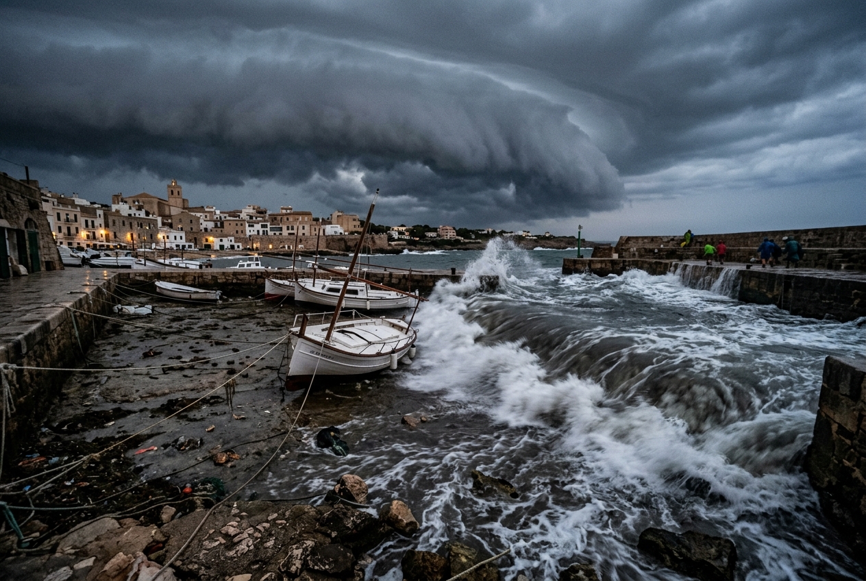
On a sweltering July afternoon along the sheltered inlet of a deep-water harbor, the air hangs motionless, saturated with humidity and the brackish tang of low tide. The water’s surface is an unbroken sheet of slate gray, reflecting a sky that has turned from pale afternoon azure to an eerie, bruised charcoal along the western horizon. Cicadas buzz in the littoral scrub, their steady drone suddenly cut short as an unnatural stillness falls over the coast. Then, the sensations arrive in quick, disorienting succession: a prickling coolness across the back of the neck, the unmistakable, sharp scent of ozone mixing with rain-splashed asphalt, and a sudden, physical sensation of fullness in the inner ear—the subtle, distinct popping sensation familiar to anyone descending rapidly in an elevator.
Along the horizon, an imposing shelf cloud—a dark, striated cylinder of condensed vapor known to meteorologists as an arcus—marches eastward like a suspended continent. Yet beneath this brooding squall, well before the first heavy raindrops strike the pier, something inexplicable happens to the sea.
Without warning, the water level begins to fall with alarming swiftness. Within four minutes, the harbor basin empties as though an enormous subterranean drain has opened. Moored sailboats list sharply onto exposed mudflats; barnacle-encrusted pilings, submerged for decades, stand naked in the damp air; crabs scurry in confusion across drying gravel beds. Bystanders walk to the edge of the docks, captivated by what appears to be a sudden, localized ebbing of the tide.
  Atmospheric Squall / Pressure Pulse (Speed = U)
  ==============================================>
  ~~~~~~~~~~~~~~~~~~~~~~~~~~~~~~~~~~~~~~~~~~~~~~~ (Sea Surface)
  ----------> Oceanic Gravity Wave (Speed = c = √(gh))
  =============================================== (Sea Floor)
   [ RESONANCE CONDITION: When U ≈ c, energy continuously transfers ]
Ten minutes later, the ocean returns. A foaming, turbid wall of water surges around the harbor headland, sweeping inward with catastrophic momentum. The water rises two, three, then four meters in a matter of minutes, snapping mooring lines like dry twine, lofting fiberglass hulls onto boardwalks, and submerging quays under a violent, churning deluge. There was no submarine earthquake, no underwater landslide, and no volcanic caldera collapse. The invisible hand that seized the water column, pulled it seaward, and flung it back onto the shore was forged entirely within the turbulent physics of the lower atmosphere.
What’s Actually Happening — Plain English First
To understand how an afternoon thunderstorm can generate an ocean wave capable of mimicking a seismic tsunami, one must first dismantle the assumption that the atmosphere is weightless.
Air has mass. At sea level, a column of air one square meter in cross-section weighs approximately ten metric tons. When atmospheric conditions are calm and uniform, this invisible blanket presses down evenly across every square inch of the ocean. However, when strong thunderstorm complexes, squall lines, or atmospheric gravity waves sweep across the coast, this blanket does not rest gently. Instead, it behaves like an undulating, heavy mattress being violently thumped and dragged across the water.
       CONVECTIVE COLD POOL & PRESSURE JUMP

             [ Downdraft ]
                   |
                   v
  -----------------+-----------------  <-- High Pressure Core (ΔP ~ +3 hPa)
  ~~~~~~~~~~~~~~~~~~~~~~~~~~~~~~~~~~~  <-- Ocean Surface Depression
             \           /
              \_________/  <-- Forced Wave travels at speed c = √(gh)
Think of the atmosphere as a layered cake, where each layer possesses a different density and temperature. When an intense storm forms, a dense, chilled pocket of air—the convective cold pool—crashes down from the upper troposphere and spreads out along the Earth's surface. As this dense wedge of air moves, it acts like a giant snowplow, creating a localized spike in barometric pressure.
Now, imagine pushing your hand through the water in a shallow bathtub. If you move your hand very slowly, the water simply parts around your fingers, creating negligible disturbance. If you move your hand at lightning speed, you create superficial spray and turbulence, but little coherent wave energy. But if you move your hand at the exact, natural speed that water ripples travel across that specific depth of the tub, something remarkable occurs: your hand continually pushes the same crest of water, transferring more and more kinetic energy into the wave, causing it to swell into a miniature surge that sloshes over the edge of the tub.
This phase-matching phenomenon is known as dynamic resonance. When an atmospheric pressure pulse races across a shallow coastal sea at the exact speed at which long gravity waves naturally propagate across the sea floor, the atmosphere and the ocean become locked in a deadly energetic embrace. The atmosphere continuously feeds kinetic and potential energy into the oceanic wave packet.
When this traveling wave finally approaches a narrow, funnel-shaped harbor or bay, a second phenomenon takes over: harbor resonance. Much like blowing air across the mouth of an empty glass bottle produces a loud, resonant tone when the frequency matches the bottle’s internal geometry, the incoming oceanic surge excites the natural sloshing frequency (the seiche) of the bay. A wave that was merely ten or twenty centimeters high in the open coastal waters is transformed by geometry and momentum into a destructive, multi-meter inundation—a phenomenon classified by meteorologists and oceanographers as a meteotsunami.
The Science: Atmospheric Coupling and Hydrodynamic Amplification
To quantify the generation and propagation of these destructive ocean waves, we must explore the interplay between mesoscale atmospheric forcing, shallow-water wave kinematics, and coastal resonance. Authoritative overviews of these hazard dynamics are maintained by agencies such as the NOAA National Ocean Service and the World Meteorological Organization.
1. The Static Inverse Barometer Effect
Under purely hydrostatic equilibrium, the ocean surface adjusts to spatial variations in atmospheric pressure. A localized increase in surface air pressure depresses the water column beneath it, while a localized pressure drop allows the ocean surface to rise.
Hydrostatic Sea-Level Response (Inverse Barometer):
Δη = - ΔP / (ρ_w * g)
Where: * $\Delta \eta$ is the vertical displacement of the sea surface ($\text{m}$), * $\Delta P$ is the atmospheric pressure perturbation ($\text{Pa}$, where $1\text{ hPa} = 100\text{ Pa}$), * $\rho_w$ is the density of seawater ($\approx 1025\text{ kg/m}^3$), * $g$ is the acceleration due to gravity ($\approx 9.81\text{ m/s}^2$).
Evaluating the product of water density and gravity gives:
$$\rho_w \cdot g \approx 1025\text{ kg/m}^3 \times 9.81\text{ m/s}^2 \approx 10055\text{ N/m}^3 \approx 10^4\text{ Pa/m}$$
Thus, a static barometric pressure change of $1\text{ hPa}$ ($100\text{ Pa}$) produces an equilibrium sea-level displacement of:
$$\Delta \eta_{\text{static}} = -\frac{100\text{ Pa}}{10055\text{ Pa/m}} \approx -0.00994\text{ m} \approx -1.0\text{ cm}$$
Clearly, a static displacement of $3\text{ cm}$ cannot account for the devastating $2\text{ to }4\text{ meter}$ surges documented during events such as the rissaga of the Balearic Islands or the surges across the Great Lakes. The missing mechanism is dynamic resonance.
2. Shallow-Water Gravity Waves and Proudman Resonance
In coastal oceanography, where the wavelength $\lambda$ of the perturbation is vastly larger than the water depth $h$ ($\lambda \gg h$), the disturbance behaves as a shallow-water long wave. The intrinsic phase velocity $c$ of a shallow-water gravity wave is governed solely by water depth:
$$c = \sqrt{g \cdot h}$$
When an atmospheric disturbance—such as a mesoscale gravity wave, an undular bore, or a convective gust front—propagates across the water surface with translation speed $U$, it continuously exerts a moving spatial pressure gradient force.
In 1929, British oceanographer Joseph Proudman derived the dynamic response of a semi-infinite water channel to a moving atmospheric pressure jump. The dynamic amplification factor $R$, often termed the Proudman resonance factor, dictates the ratio between the dynamically forced wave amplitude $\eta_{\text{dynamic}}$ and the static inverse barometer displacement $\eta_{\text{static}}$:
$$R = \frac{1}{\left| 1 - \left( \frac{U}{\sqrt{g \cdot h}} \right)^2 \right|} = \frac{1}{\left| 1 - Fr^2 \right|}$$
Where $Fr = U / \sqrt{gh}$ represents the hydrodynamic Froude number of the atmospheric forcing. Comprehensive derivations of this phenomenon are detailed in coastal hydrodynamic literature and synthesized within Proudman Resonance on Wikipedia and broader research on Meteotsunamis.
PROUDMAN RESONANCE AMPLIFICATION FACTOR (R)
------------------------------------------------------
Froude Number (Fr = U/c)   Theoretical R   Physical State
------------------------------------------------------
0.20                       1.04            Subcritical (Static-like)
0.50                       1.33            Subcritical (Weak dynamic)
0.80                       2.78            Subcritical (Moderate amplification)
0.95                       10.26           Near-Resonant (High amplification)
1.00                       ∞ (Linear t)    Perfect Proudman Resonance
1.05                       9.76            Supercritical (Near-Resonant)
1.50                       0.80            Supercritical (Decoupled)
------------------------------------------------------
Worked Numerical Example: The Anatomy of a Proudman Resonance Event
Let us model a typical summer squall line crossing an epicontinental shelf or shallow embayment:
- Bathymetric Depth: $h = 25\text{ meters}$.
- Oceanic Gravity Wave Speed: $$c = \sqrt{9.81\text{ m/s}^2 \times 25\text{ m}} = \sqrt{245.25} \approx 15.66\text{ m/s} \approx 56.4\text{ km/h} \approx 30.4\text{ knots}$$
- Atmospheric Disturbance Speed: The convective gust front advances at $U = 54.0\text{ km/h} \approx 15.0\text{ m/s}$.
- Froude Number Calculation: $$Fr = \frac{U}{c} = \frac{15.0\text{ m/s}}{15.66\text{ m/s}} \approx 0.958$$
- Dynamic Amplification Factor: $$R = \frac{1}{\left| 1 - (0.958)^2 \right|} = \frac{1}{\left| 1 - 0.9178 \right|} = \frac{1}{0.0822} \approx 12.16$$
If the convective downdraft generates a transient atmospheric pressure jump of $\Delta P = 3.5\text{ hPa}$, the static water displacement would be only:
$$\Delta \eta_{\text{static}} \approx 3.5\text{ cm} = 0.035\text{ m}$$
However, subjected to near-perfect Proudman resonance ($Fr \approx 0.96$), the open-water wave crest is dynamically amplified to:
$$\eta_{\text{open-water}} = R \times \Delta \eta_{\text{static}} = 12.16 \times 0.035\text{ m} \approx 0.426\text{ m} \approx 42.6\text{ cm}$$
While a $43\text{ cm}$ wave in the open coastal zone is noticeable, it is rarely catastrophic on its own. The final, destructive transformation occurs as this amplified wave enters a semi-enclosed coastal geometry.
3. Harbor Resonance and Topographic Funneling
When the open-water wave reaches the coastline, shoaling concentrates its energy, compressing the wavelength and increasing its height according to Green's Law ($H \propto h^{-1/4}$). Upon entering an inlet, bay, or harbor, the wave encounters the basin's natural eigenmodes of oscillation.
QUARTER-WAVE HARBOR RESONANCE
Head (Closed)                                       Mouth (Open)
|                                                              |
|=====\                                                        |
|      \                                                       |
|       \______________________________________________________|
| Node (Maximum Velocity)              Antinode (Maximum Elevation)
|<----------------- Harbor Length (L) ------------------------>|
For an elongated, semi-enclosed harbor open at one end and closed at the other (such as Port de Ciutadella in Menorca or long bays in the Great Lakes), the fundamental standing wave mode—the quarter-wave resonator—has an eigenperiod $T_0$ governed by Merian’s formula:
$$T_0 = \frac{4L}{\sqrt{g \cdot h_m}}$$
Where: * $L$ is the length of the harbor channel ($\text{m}$), * $h_m$ is the mean depth of the channel ($\text{m}$).
If the spectral peak of the incoming atmospheric wave train or open-ocean wave packet matches the fundamental period $T_0$ of the harbor, Helmholtz resonance is established. Energy accumulates within the basin over several successive wave cycles with minimal dissipative loss.
CALCULATION CALLOUT: HARBOR RESONANCE IN A 1.2 KM INLET
-------------------------------------------------------------------------
Channel Length (L)  : 1,200 m
Mean Depth (h_m)     : 5.5 m
Phase Velocity (c)  : √(9.81 * 5.5) = 7.34 m/s
Fundamental Period  : T_0 = (4 * 1200 m) / (7.34 m/s) = 4800 / 7.34 ≈ 654 s (10.9 min)

Result: An incoming wave train with an energy period of ~11 minutes will
resonate violently inside this inlet, amplifying the open-water 43 cm wave
by a factor of 4 to 8, producing harbor surges exceeding 3.0 to 3.5 meters!
-------------------------------------------------------------------------
Practical Outdoor Guidance
Meteotsunamis are notoriously dangerous because they frequently occur during fair-weather windows immediately preceding a storm, or strike coasts located dozens of kilometers away from the parent convective cell. For coastal residents, mariners, fishermen, and emergency managers, recognizing early atmospheric precursors can provide life-saving minutes of warning. Technical tracking methodologies and storm monitoring guidelines can be reviewed at the Met Office.
             METEOTSUNAMI RAPID DIAGNOSTIC WORKFLOW

 [ Sky Observation ] ----> Roll Cloud / Arcus / Dark Squall Line
          |
 [ Microbarograph ]  ----> Rapid Jump: ΔP > 2 hPa in < 10 minutes
          |
 [ Radar Doppler ]   ----> Cell Motion Speed U matches local c = √(gh)
          |
 [ Harbor Water ]    ----> Uncharacteristic rapid drawdown or surging
          v
 [ ACTION: EVACUATE LOW DOCKS, BASINS, AND EXPOSED HARBORS IMMEDIATELY ]
1. What to Look for in the Sky
- The Arcus Signature: A low, sharp, dark shelf cloud spanning the horizon indicates an aggressive density current (gust front). The sharper and more linear the shelf cloud, the more coherent the advancing cold pool.
- Undulatus Cloud Formations: Parallel, rib-like wave patterns across the cloud deck signify trapped atmospheric gravity waves propagating along a mid-level inversion layer. These waves often modulate the surface pressure field with exact periodicity.
- Abrupt Atmospheric Stagnation: A sudden, eerie cessation of ambient coastal breeze followed by a rapid shift of 90° to 180° in wind direction indicates the passage of a mesoscale pressure boundary.
2. Instrument Readings to Monitor
- Digital Microbarographs: Standard weather stations often record pressure every 30 to 60 minutes, which completely misses meteotsunami triggers. Configure your barograph to log at 1-minute intervals. Watch for a pressure tendency spike exceeding $\Delta P \ge 1.5\text{ to }3.0\text{ hPa}$ within a 5- to 15-minute window.
- Thermometer Trends: A sudden temperature drop of $3^\circ\text{C to }8^\circ\text{C}$ ($5^\circ\text{F to }15^\circ\text{F}$) coincident with a pressure spike confirms the arrival of a density-driven convective cold pool.
- Doppler Radar Velocity: Track the speed of approaching convective lines. Using the equation $c = \sqrt{gh}$, determine the wave speed of your local offshore waters. For continental shelves with depths of $15\text{ to }40\text{ meters}$, squalls traveling between 45 and 75 km/h (25 to 40 knots) represent maximum Proudman resonance hazards.
Today’s Meteorological Rule of Thumb
When a fast-moving squall line approaches shallow coastal waters at highway speeds (45–75 km/h), treat any sudden, unprompted drainage of harbor water or rapid barometric jump greater than 2 hPa as an immediate tsunami warning: dynamic atmospheric resonance has coupled with the sea floor, and a destructive ocean surge will follow within minutes.