Polar Lows & Arctic Maritime Cyclogenesis: How Extreme Air-Sea Fluxes and Upper Troughs Unleash High-Latitude Storms

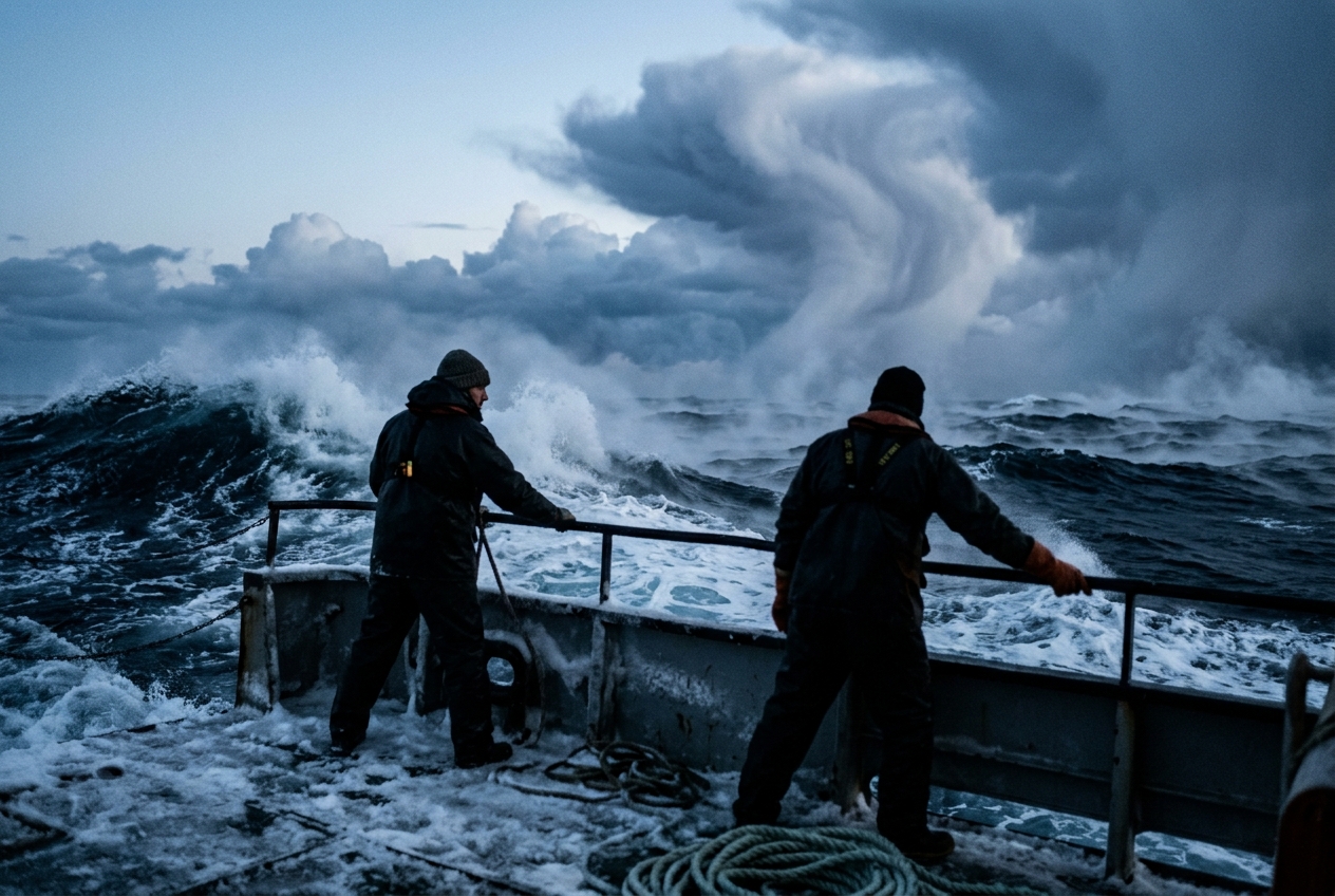
Sixty miles north of Norway’s North Cape, across the churning, ink-black waters of the Barents Sea, winter maritime navigation is defined by an eerie, fragile equilibrium. On a mid-January afternoon, under the perpetual twilight of the polar night, the atmosphere initially seems suspended in crystalline stasis. The barometer rests near a comfortable 1012 hectopascals. The wind is a moderate, biting 15-knot northerly that carries the dry, pine-needle chill of the Svalbard ice shelf. Sea spray freezes almost instantly upon hitting the steel bulwarks of a vessel, leaving a thin glaze of rime.

Then, within the span of barely twenty minutes, the maritime boundary layer begins to unravel.

The mercury in the barograph does not merely fall; it plunges in a precipitous, vertical descent, shedding six hectopascals in less than an hour. The horizon to the north vanishes behind an ominous, slate-grey curtain that rolls across the water like an encroaching mountain range. As the wall of cloud makes landfall over the ship, the wind veers sharply by eighty degrees and screams into a sustained 50-knot gale, with localized gusts ripping across the wave crests at hurricane force.

The air transforms into a blinding, whiteout maelstrom of convective graupel and dense snow. Ocean swells, previously orderly and rhythmic, are torn into chaotic, foaming peaks known as spindrift, while the surface of the sea appears to boil—a phenomenon known to mariners as "Arctic sea smoke." This is not an ordinary winter gale or the predictable edge of an Atlantic depression. It is the sudden, violent genesis of a polar low: an intense, sub-synoptic maritime cyclone whose compact vortex and thermodynamic engine mirror the structural majesty of a tropical hurricane in the sub-zero expanse of the high latitudes.

       POLAR TROPOSPHERE & POLAR LOW GENESIS

  Upper Troposphere (~500 hPa / ~5 km altitude)
  Cold Core Anomaly / PV Intrusion [ T ≈ -40°C to -45°C ]
  -------------------vvvvvvvvvvvvvvvv-------------------
                      \              /  <-- Dynamic Upper Forcing
                       \  Vorticity /
                        \  Anomaly /
                         \        /
  Mid-Level Convection    \      /      Intense Updrafts
  & Latent Heat Release    \    /       & Snow Bands
                           ( ^^ )
                          ( ^^^^ )
                         ( ^^^^^^ )
  ------------------------------------------------------
  Marine Boundary Layer: Extreme Air-Sea Fluxes (Q_H + Q_E)
  Open Ocean Surface [ SST ≈ +2°C to +5°C ]
  ~~~~~~~~~~~~~~~~~~~~~~~~~~~~~~~~~~~~~~~~~~~~~~~~~~~~~~

1. What’s Actually Happening — Plain English First

To understand why the high Arctic suddenly unleashes these violent, localized tempests, think of the atmosphere as a layered cake where stability depends entirely on temperature and buoyancy. Under normal, calm conditions, air is stacked neatly: heavy, dense, cold air rests close to the ground or water, while progressively lighter, thinner air sits above it. When undisturbed, this arrangement resists vertical movement. Air parcels have no natural inclination to rise, meaning the sky remains quiet.

A polar low overturns this stability with catastrophic efficiency. The process begins when an immense reservoir of ultra-frigid continental air—often cooled to $-25^\circ\text{C}$ or lower over the permanent Arctic sea ice—is driven southward over the ice edge by large-scale weather patterns. Suddenly, this frozen air mass finds itself flowing over the open waters of the Norwegian, Barents, or Labrador Seas, which are kept relatively warm ($+2^\circ\text{C}$ to $+6^\circ\text{C}$) by the northern extensions of the Gulf Stream.

        THE ARCTIC "HOT SKILLET" INSTABILITY

  Frigid Continental Arctic Air (-25°C)
  =======> [Sea Ice Edge] =======>
                                   \
   Air advects over warm water      \   Vigorous Convective Plumes
                                     \  (Rapid Upward Chimney Effect)
                                    _ \ _  _   _   _
                                   ( ) ( )( ) ( ) ( )
  ~~~~~~~~~~~~~~~~~~~~~~~~~~~~~~~~~~~~~~~~~~~~~~~~~~~~~~~~
  Relatively Warm Ocean Surface (+4°C)
  [ Ocean acts like a boiling bath beneath a frozen room ]

Imagine opening the door of a walk-in commercial freezer directly over a bubbling, steaming hot tub. The moment the sub-zero air meets the warm water, heat and moisture erupt violently into the lowest layer of the atmosphere. The ocean acts like a massive, heated radiator beneath a freezing ceiling. Because warm, moisture-laden air is far less dense than the dry, icy air sitting directly on top of it, the heated air shoots upward in powerful, buoyant thermal chimneys.

While mid-latitude winter storms (such as Atlantic low-pressure systems or Nor'easters) draw their primary fuel from the broad clash of horizontal temperature zones across thousands of kilometres—a mechanism known as baroclinicity—polar lows frequently behave like miniature tropical hurricanes. Once triggered, they can transition into self-sustaining heat engines.

The rising air cools, causing the moisture evaporated from the sea to condense into snow and graupel, releasing vast reservoirs of hidden heat (latent heat) directly into the storm’s spinning core. This internal heating causes pressure at the sea surface to plummet even further, pulling in surrounding winds at higher speeds, which in turn scoops up even more heat and moisture from the waves. Under the right conditions, this feedback loop wraps convective snow bands tightly around an eerily calm, cloud-free eye.

2. The Science: Thermodynamic Fluxes and Dynamic Amplification

For atmospheric scientists and physical oceanographers, the polar low represents one of the most extreme thermodynamic interactions on Earth. The rapid intensification of these systems is governed by two complementary mechanisms: massive turbulent surface energy exchange at the lower boundary, and dynamic potential vorticity (PV) anomalies aloft.

The Engine Room: Bulk Aerodynamic Heat Fluxes

The primary energy reservoir initiating a polar low is the combined total surface turbulent heat flux, composed of sensible heat flux ($Q_H$)—direct thermal conduction and warm convection—and latent heat flux ($Q_E$), which represents the energy transported via evaporated water vapor.

The magnitude of this energy transfer from sea to air is quantified through the Bulk Aerodynamic Formulas:

$$Q_{total} = Q_H + Q_E = \rho c_p C_H U_{10} (T_{sfc} - T_a) + \rho L_v C_E U_{10} (q_{sfc} - q_a)$$

Where: * $\rho$ is the surface air density ($\text{kg/m}^3$) * $c_p$ is the specific heat capacity of dry air at constant pressure ($\approx 1005\text{ J}\cdot\text{kg}^{-1}\text{K}^{-1}$) * $L_v$ is the latent heat of vaporization of water ($\approx 2.50 \times 10^6\text{ J/kg}$) * $C_H$ and $C_E$ are the dimensionless bulk transfer coefficients for sensible heat and moisture (typically $\approx 1.3 \times 10^{-3}$ to $1.8 \times 10^{-3}$ in unstable, high-wind marine regimes) * $U_{10}$ is the sustained wind speed at standard 10-metre anemometer height ($\text{m/s}$) * $T_{sfc}$ and $T_a$ are the sea surface temperature and air temperature at 10 metres, respectively * $q_{sfc}$ and $q_a$ are the saturation specific humidity at sea surface temperature and the actual ambient air specific humidity, respectively

Worked Example: Energy Transfer in a Barents Sea Outbreak

Let us examine realistic meteorological data collected during an Arctic Cold Air Outbreak (CAO) over the south-western Barents Sea:

• Surface Air Density ($\rho$): $1.32\text{ kg/m}^3$ (frigid air is exceptionally dense)
• 10-metre Wind Speed ($U_{10}$): $20.0\text{ m/s}$ (approx. 39 knots, near-gale)
• Bulk Transfer Coefficients ($C_H \approx C_E$): $1.5 \times 10^{-3}$
• Sea Surface Temperature ($T_{sfc}$): $+4.0^\circ\text{C}$ ($277.15\text{ K}$)
• 10-metre Air Temperature ($T_a$): $-16.0^\circ\text{C}$ ($257.15\text{ K}$)
• Air-Sea Temperature Difference ($\Delta T = T_{sfc} - T_a$): $+20.0\text{ K}$
• Surface Saturation Specific Humidity ($q_{sfc}$ at $+4^\circ\text{C}$): $5.1 \times 10^{-3}\text{ kg/kg}$
• Ambient Air Specific Humidity ($q_a$ at $-16^\circ\text{C}$, 75% RH): $0.8 \times 10^{-3}\text{ kg/kg}$
• Humidity Gradient ($\Delta q = q_{sfc} - q_a$): $4.3 \times 10^{-3}\text{ kg/kg}$

Step 1: Calculate the Sensible Heat Flux ($Q_H$) $$Q_H = 1.32 \times 1005 \times (1.5 \times 10^{-3}) \times 20.0 \times 20.0$$ $$Q_H = 1.32 \times 1005 \times 0.030 \times 20.0 \approx 795.96\text{ W/m}^2$$

Step 2: Calculate the Latent Heat Flux ($Q_E$) $$Q_E = 1.32 \times (2.50 \times 10^6) \times (1.5 \times 10^{-3}) \times 20.0 \times (4.3 \times 10^{-3})$$ $$Q_E = 4950 \times 20.0 \times 0.0043 \approx 425.70\text{ W/m}^2$$

Step 3: Sum Total Marine Boundary Layer Energy Flux ($Q_{total}$) $$Q_{total} = Q_H + Q_E = 795.96 + 425.70 = 1221.66\text{ W/m}^2$$

The Instability Threshold: The $SST - T_{500\text{hPa}}$ Metric

Empirical and theoretical analyses maintained by organizations like the World Meteorological Organization (WMO) and the European Centre for Medium-Range Weather Forecasts (ECMWF) establish a vital operational rule for polar low cyclogenesis. Because the Arctic troposphere is compressed into a shallow depth of only 7 to 9 kilometres (compared to 16 km in the tropics), deep convection requires an exceptionally steep environmental lapse rate.

The canonical instability threshold for polar low development across the Nordic Seas and Gulf of Alaska is defined as:

$$SST - T_{500\text{hPa}} \ge 44^\circ\text{C}$$

When the temperature differential between the unfrozen sea surface and the middle troposphere (approximately 5,000 metres altitude, corresponding to the 500 hPa pressure surface) exceeds $44^\circ\text{C}$, the vertical temperature lapse rate ($\Gamma = -\partial T / \partial z$) approaches or exceeds the dry adiabatic lapse rate ($\approx 9.8^\circ\text{C/km}$) through the lower-to-middle levels.

Under these conditions, convective inhibition (CIN) is obliterated, allowing sea-surface air parcels to accelerate unhindered into the upper troposphere, creating deep convective chimneys.

       VERTICAL LAPSE RATE PROFILE DURING ARCTIC OUTBREAK

  Altitude (km)
     ^
  8  |   Tropopause / Upper Anomaly [ T ≈ -45°C ]
  7  |           *
  6  |          *  <-- Convective Equilibrium Curve
  5  |   500 hPa level [ T <= -40°C ]
  4  |        *
  3  |       *     STEEP LAPSE RATE (Gamma > Gamma_m)
  2  |      *      Rapid Uncontrolled Buoyant Ascent
  1  |     *
  0  |____*_____________________________> Temperature (°C)
        -40°C   -30°C   -20°C   -10°C    0°C   +4°C (SST)

Upper-Tropospheric Potential Vorticity (PV) and Reverse Shear

While surface heat fluxes supply the fuel, the trigger is usually pulled in the upper atmosphere. Polar lows are frequently initiated by the advection of an upper-level Potential Vorticity (PV) anomaly—a downward intrusion of stratospheric air rich in potential vorticity ($PV > 2.0\text{ PVU}$, where $1\text{ PVU} = 10^{-6}\text{ m}^2\text{s}^{-1}\text{K kg}^{-1}$).

Ertel's Potential Vorticity in isentropic coordinates is expressed as:

$$P = -g \left( \zeta_\theta + f \right) \frac{\partial \theta}{\partial p}$$

Where $\zeta_\theta$ is relative vorticity evaluated on an isentropic (constant potential temperature $\theta$) surface, $f$ is the Coriolis parameter ($2\Omega \sin \phi$), and $\partial \theta / \partial p$ represents static stability.

When a dry stratospheric extrusion penetrates down toward the 600–500 hPa level, it imposes strong cyclonic rotation aloft and induces strong upward dynamic motion ahead of its path. When this dynamically forced ascent aligns directly over a marine boundary layer primed with $>1000\text{ W/m}^2$ of heat flux, rapid cyclogenesis occurs.

Furthermore, polar lows frequently mature in reverse-shear baroclinic environments. In typical mid-latitude storms, the thermal wind vector aligns parallel to the low-level steering flow (forward shear).

In Arctic outbreaks, the coldest air often lies to the south or south-west of the developing mesoscale center due to the geometry of retreating ice sheets and topography. This causes the environmental wind to decrease or reverse direction with height, focusing vertical vorticity into a compact, tightly wound, axisymmetric core rather than spreading the system along a broad, frontal boundary.

Morphological Classification: Spiraliform vs. Comma-Shaped

High-resolution polar-orbiting satellite passes curated by the National Oceanic and Atmospheric Administration (NOAA) and the Met Office reveal that polar lows fall into two primary structural archetypes:

  ===================================================================
                       POLAR LOW MORPHOLOGIES
  ===================================================================

    1. SPIRALIFORM (Quasi-Tropical)     2. COMMA-SHAPED (Baroclinic)
             .-""""-.                             .---.
           .'  _  _  '.                         .'     '.
          /   (o)(o)   \                       /   / \   \
         |      ()      |                     |   |   |   |
         |   \______/   |                      \   \ /   /
          \   CONVECT. /                        '.     .'  <-- Frontal
           '.  BANDS .'                           '---'       Band
             '-....-'                               \  \
                ||                                   \  \
          * Symmetrical Eye                    * Asymmetric Tail
          * Pure WISHE/CISK Dominant           * Baroclinic Shear Driven
          * Compact (100–300 km)               * Mesoscale Front (300–600 km)
  ===================================================================

1. Spiraliform Polar Lows: * Dynamics: Dominated by axisymmetric convective processes akin to the Wind-Induced Surface Heat Exchange (WISHE) and Conditional Instability of the Second Kind (CISK) mechanisms. * Structural Anatomy: Characterized by a distinct, calm, cloud-free central "eye" surrounded by tight convective cloud walls and spiral rain/snow bands. Horizontal diameter is typically compact (100 to 300 kilometres). * Environment: Occurs in weak ambient baroclinic shear over open waters with deep thermal instability.

2. Comma-Shaped Polar Lows: * Dynamics: Primarily driven by low-to-mid level baroclinic instability and localized mesoscale shear vorticity along cold-air boundaries. * Structural Anatomy: Resembles a miniature mid-latitude synoptic system, featuring an elongated convective "head" and a distinct cold-frontal "tail" wrapping into the vortex. * Environment: Common along the margins of coastal topography or the marginal ice zone (MIZ) where strong horizontal temperature gradients persist.

For further reading on high-latitude cyclogenesis taxonomy, explore the Wikipedia Polar Low Reference and meteorological archives maintained by the National Snow and Ice Data Center (NSIDC).

3. Practical Outdoor Guidance for Mariners and Coastal Observers

Because polar lows develop beneath the horizontal resolution grid of many global numerical weather prediction models, they remain notorious for evading standard long-range forecasts. Coastal communities along northern Norway, Iceland, the British Isles, Alaska, and Japan (the Sea of Japan "polar cold vortex lows") must rely on direct atmospheric observations and high-frequency updates.

What to Look for in the Sky

• Arctic Sea Smoke (Steam Fog): The sudden appearance of dense, whispy condensation plumes rising directly off the water surface indicates that the air-sea temperature gradient ($\Delta T$) has exceeded critical instability levels ($>15^\circ\text{C}$ differential).
• Convective Snow Rollers and Cloud Streets: Parallel bands of cumulus clouds (cloud streets) extending south from the ice pack indicate that massive sensible heat exchange is under way. If these linear bands begin to bend, curl, or wrap into a cyclonic spiral on the horizon, mesoscale cyclogenesis has initiated.
• The "Lead Curtain": Unlike the slow, diffuse overcast preceding warm fronts, a polar low's convective snow squall approaches as a solid, dark, shelf-like wall stretching from the sea surface into the middle troposphere.

       ANATOMY OF AN APPROACHING POLAR LOW SQUALL WALL

  Altitude
     ^
  3km|                     [ DENSE CUMULONIMBUS ROLL ]
     |                       .-''''-.
  2km|                      / Convect\
     |                     |  Graupel |
  1km|                     |  & Snow  |   Turbulent Roll Cloud
     |    Clear / Calm     \  Tower   /  /
  0km|________Zone__________\________/__v__________________
     |                      |        |  Heavy Whiteout
     |<-- Barometer Drops   | SQUALL |  Wind Gusts > 50 kts
     |    (Pre-Vortex)      |  FRONT |  Freezing Spray
  ~~~|~~~~~~~~~~~~~~~~~~~~~~|~~~~~~~~|~~~~~~~~~~~~~~~~~~~~~

Critical Instrument Signatures

1. The Barometer: Any barometric pressure drop exceeding $3.0\text{ hPa}$ in a 3-hour period at high latitudes is an alert; a drop exceeding $2.0\text{ hPa}$ within a single hour signifies immediate proximity to a developing polar low core.
2. The Thermometer / Psychrometer: A counter-intuitive signature: as the polar low's core passes over, local surface air temperatures may briefly rise several degrees due to the intense upwelling of marine boundary layer heat and latent heat release, before plunging violently as the system's western flank sweeps cold Arctic air behind it.
3. Wind Shifts: Watch for rapid wind directional shear. A backing wind (turning counter-clockwise from south-westerly to south-easterly, then snapping violently northerly) indicates that the eye of a polar low is passing just to your east.

Superstructure Icing: The Maritime Danger

The lethal hallmark of the polar low is rapid superstructure icing. When 40 to 60-knot winds churn open sea water at temperatures between $-1.5^\circ\text{C}$ and $+2.0^\circ\text{C}$ into fine spray, and the ambient air sits below $-10^\circ\text{C}$, the spray freezes immediately upon contact with a vessel's hull, masts, and rigging.

Accumulations can exceed 3 to 5 centimetres of solid ice per hour. This top-heavy accumulation rapidly raises the ship's center of gravity ($CG$), degrading the metacentric height ($GM$) and leading to sudden, catastrophic capsizing.

+-------------------------------------------------------------------------+
|                  SUMMARY: SYNOPTIC VS. POLAR LOW CYCLONES               |
+-------------------------------------------------------------------------+
| Feature              | Mid-Latitude Depression | Polar Low Mesocyclone  |
+----------------------+-------------------------+------------------------+
| Horizontal Scale     | 1,000 – 3,000 km        | 100 – 500 km           |
| Primary Fuel Source  | Horizontal Baroclinicity| Air-Sea Fluxes + Latent|
| Lifetime             | 3 – 7 Days              | 12 – 36 Hours          |
| Eye Structure        | Extremely Rare          | Common (Spiraliform)   |
| Deepest Instability  | Frontal Boundaries      | Core Convection (WISHE)|
| Prediction Window    | 4 – 7 Days in Advance   | 3 – 18 Hours Notice    |
+-------------------------------------------------------------------------+

4. Today’s Meteorological Rule of Thumb

External References and Authoritative Resources

• National Oceanic and Atmospheric Administration (NOAA) — Global satellite imagery and high-latitude marine forecasting tools.
• World Meteorological Organization (WMO) — Guidelines on mesoscale polar weather systems and Arctic observation networks.
• European Centre for Medium-Range Weather Forecasts (ECMWF) — State-of-the-art reanalysis of polar cold air outbreaks and mesocyclone predictability.
• UK Met Office Meteorological Services — Educational resources on polar low formation, fronts, and marine safety.
• National Snow and Ice Data Center (NSIDC) — Cryospheric boundaries, sea ice margins, and polar atmospheric research.