Hypsometric Equation & Geopotential Thickness: How Mean Virtual Temperature Governs Atmospheric Layer Expansion and Synoptic Ridge Heights
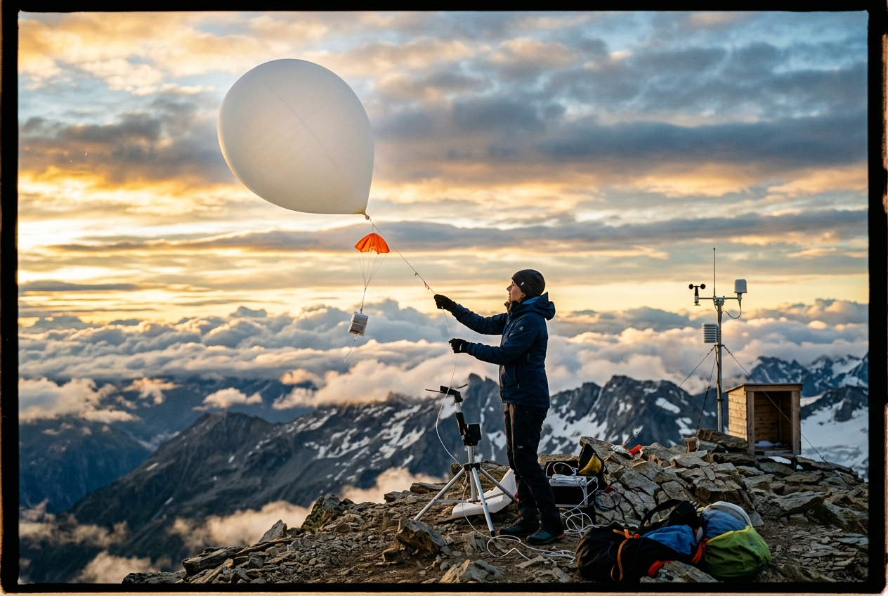
As you pause to check your wrist-mounted barometric altimeter, an odd anomaly catches your eye. You have not descended a single foot, yet the digital display insists you have climbed thirty metres in the last twenty minutes. The air pressure is dropping rapidly, and the thermometer in your pack pocket reads $-4^\circ\text{C}$. Within the hour, the gentle mist transforms into stinging graupel, and then into large, feather-light snowflakes that blanket the scree.
Unbeknownst to the casual observer, you are standing inside an immense thermodynamic engine. The invisible vertical column of air resting above your head is shrinking, compressing downward like a chilled bellows. This invisible architectural shift of the atmosphere—the thermal expansion and contraction of air layers—is governed by one of the most fundamental relationships in dynamic meteorology: the hypsometric equation.
What’s Actually Happening: The Atmospheric Accordion
To make sense of why the sky behaves this way, think of the atmosphere not as a static ocean of air, but as an enormous, multi-tiered accordion.
Air is composed of trillions of microscopic gas molecules bouncing against one another. When air warms, those molecules absorb kinetic energy, dart around faster, and push each other farther apart. The air becomes less dense and expands upward. Conversely, when an Arctic air mass sweeps in, the molecules lose kinetic energy, slow down, and pack tightly together under the weight of gravity. The entire column of air cools, densifies, and collapses toward the Earth's surface.
       WARM AIR MASS (Expanded)              COLD AIR MASS (Contracted)
   500 hPa -------------------------     500 hPa ------------------------- (Lower Height)
          |                         |            |                         |
          |    THICK LAYER          |            |    THIN LAYER           |
          |    (High Thickness)     |            |    (Low Thickness)      |
          |    Molecules dispersed  |            |    Molecules compressed |
          |                         |            |                         |
  1000 hPa =========================    1000 hPa =========================
Meteorologists map this behavior by tracking isobaric surfaces—invisible, undulating sheets in the atmosphere where the atmospheric pressure is exactly equal everywhere. Instead of asking what the pressure is at a fixed height of 5,000 metres, forecasters ask: At what height above sea level does the pressure drop to 500 hectopascals (hPa)?
If the air between sea level (roughly $1000\text{ hPa}$) and the mid-troposphere ($500\text{ hPa}$) is tropical and warm, that layer will be swollen and tall; you might have to climb 5,700 metres before the pressure drops to $500\text{ hPa}$. If that same layer is occupied by polar air, it shrinks, and you might reach the $500\text{ hPa}$ level at just 5,100 metres.
The vertical distance between two pressure surfaces is called geopotential thickness. Thickness is nothing more or less than a giant, atmospheric thermometer: the thicker the layer, the warmer the average temperature of that air column.
There is one further subtlety that every meteorologist must account for: humidity. Water vapor ($H_2O$) has a molecular weight of roughly $18\text{ g/mol}$, whereas dry air (dominated by nitrogen and oxygen) averages about $28.97\text{ g/mol}$. Because a volume of gas at a given temperature and pressure contains the same number of molecules regardless of their species (as described by Avogadro's Law), introducing lighter water vapor molecules actually makes moist air less dense than dry air at the same temperature. Meteorologists resolve this by calculating the virtual temperature ($T_v$)—the temperature that completely dry air would need to have in order to match the exact density of moist air.
The Mathematical Foundation: Deriving the Hypsometric Equation
To understand how professional forecasters turn these physical principles into operational predictions, we must derive the quantitative relation linking pressure, temperature, and height from first principles.
1. The Hydrostatic Balance
Consider a static vertical parcel of air with cross-sectional area $A$ and infinitesimal thickness $dz$. The mass of this parcel is $dm = \rho A dz$, where $\rho$ is the atmospheric density. The downward gravitational force acting on this parcel is $dF_g = dm \cdot g = \rho g A dz$.
For the parcel to remain in vertical equilibrium without accelerating violently upward or downward, this downward gravitational weight must be precisely balanced by the vertical pressure gradient force: the upward push from higher pressure at the base ($p$) versus slightly lower pressure at the top ($p + dp$):
$$(p)A - (p + dp)A = \rho g A dz$$
Simplifying this yields the classical Hydrostatic Equation:
$$\frac{dp}{dz} = -\rho g \quad \implies \quad dp = -\rho g dz$$
This fundamental relationship, monitored closely across global observation networks managed by the World Meteorological Organization (WMO), states that pressure must decrease monotonically with increasing height.
                  p + dp  (Top of parcel: Lower Pressure)
                 +-----------------------+
                 |       ^               |
                 |       | Upward PGF    |
           dz    |       |               |  Gravity (Down)
                 |       v  Weight (dm*g)|      |
                 |                       |      v
                 +-----------------------+
                     p    (Base of parcel: Higher Pressure)
2. The Equation of State for Moist Air
Dry air obeys the ideal gas law: $p = \rho_d R_d T$, where $R_d = 287.058\text{ J kg}^{-1}\text{ K}^{-1}$ is the specific gas constant for dry air. In the real troposphere, moisture reduces overall density. We incorporate this by introducing the virtual temperature ($T_v$):
$$p = \rho R_d T_v$$
Where $T_v$ can be accurately approximated from dry-bulb temperature $T$ (in Kelvin) and specific humidity $q$ (in $\text{kg/kg}$) as:
$$T_v \approx T(1 + 0.608 q)$$
Rearranging for density $\rho$:
$$\rho = \frac{p}{R_d T_v}$$
3. Integrating the Hypsometric Equation
Substituting this expression for density into the hydrostatic equation yields:
$$dp = -\left(\frac{p}{R_d T_v}\right) g dz$$
Separating variables so that all pressure terms are on the left and geometric terms are on the right:
$$\frac{dp}{p} = -\frac{g}{R_d T_v} dz$$
In meteorological practice, gravity varies subtly with latitude and altitude. To eliminate this variation, atmospheric scientists define geopotential height ($Z$), normalized by standard sea-level gravity $g_0 = 9.80665\text{ m s}^{-2}$, such that $g dz = g_0 dZ$. Making this substitution:
$$\frac{dp}{p} = -\frac{g_0}{R_d T_v} dZ$$
We now integrate this differential equation vertically between a lower isobaric boundary $p_1$ at geopotential height $Z_1$, and an upper isobaric boundary $p_2$ at geopotential height $Z_2$ (where $p_1 > p_2$ and $Z_2 > Z_1$):
$$\int_{p_1}^{p_2} \frac{dp}{p} = -\frac{g_0}{R_d} \int_{Z_1}^{Z_2} \frac{dZ}{T_v}$$
By applying the mean value theorem, we can pull the layer-averaged mean virtual temperature, denoted as $\bar{T}_v$, out of the integral:
$$\ln\left(\frac{p_2}{p_1}\right) = -\frac{g_0}{R_d \bar{T}_v} (Z_2 - Z_1)$$
Multiplying both sides by $-1$ reverses the natural logarithm argument ($\ln(p_1/p_2)$), allowing us to solve directly for the layer thickness $\Delta Z = Z_2 - Z_1$:
$$\Delta Z = Z_2 - Z_1 = \left( \frac{R_d \bar{T}_v}{g_0} \right) \ln\left(\frac{p_1}{p_2}\right)$$
This is the celebrated Hypsometric Equation. It proves mathematically that the thickness of an atmospheric layer bounded by two isobaric surfaces is strictly proportional to the mean virtual temperature ($\bar{T}_v$) of that layer.
Synoptic Meteorology: The 1000–500 hPa Thickness and the 540 dam Line
In operational forecasting at agencies like the National Oceanic and Atmospheric Administration (NOAA) and the UK Met Office, thickness maps represent one of the most powerful diagnostic tools for diagnosing thermal advection and identifying precipitation boundaries.
The most widely scrutinized thickness product is the $1000\text{--}500\text{ hPa}$ layer thickness. This spans roughly the lower half of the atmosphere's total mass—from near sea level up to roughly $5.5\text{ km}$ altitude.
Let us evaluate the hypsometric constant for this specific layer. Setting $p_1 = 1000\text{ hPa}$ and $p_2 = 500\text{ hPa}$:
$$\ln\left(\frac{1000}{500}\right) = \ln(2) \approx 0.693147$$
The thickness proportionality factor becomes:
$$C = \frac{R_d \ln(2)}{g_0} = \frac{287.058 \times 0.693147}{9.80665} \approx 20.288\text{ m K}^{-1}$$
Thus, the thickness of the $1000\text{--}500\text{ hPa}$ layer simplifies to the linear relation:
$$\Delta Z_{1000-500} \approx 20.288 \times \bar{T}_v \quad (\text{in metres})$$
In synoptic meteorology, heights are traditionally reported in decametres ($\text{dam}$, where $1\text{ dam} = 10\text{ metres}$).
$$\Delta Z_{1000-500} \approx 2.0288 \times \bar{T}_v \quad (\text{in decametres})$$
+-----------------------------------------------------------------------------------+
| SYNOPTIC THICKNESS CHART (1000-500 hPa)                                           |
|                                                                                   |
|                   POLAR AIR MASS (Cold Trough)                                    |
|                   [ 516 dam ]                                                     |
|                        \                                                          |
|                         \                                                         |
|   - - - - - - - - - - -  \ - - - - - - - - - - - - - - - - - - - - - - - - - - - - |
|   CRITICAL 540 dam LINE:  * * * * * * * * * * * * * * * * * * * * * * * * * * * *  |
|   (50% Rain / 50% Snow)  / (Transition Zone: Freezing Rain, Sleet, Wet Snow)      |
|   - - - - - - - - - - - / - - - - - - - - - - - - - - - - - - - - - - - - - - - - |
|                        /                                                          |
|                   SUBTROPICAL AIR MASS (Thermal Ridge)                            |
|                   [ 564 dam ]                                                     |
+-----------------------------------------------------------------------------------+
The 540 dam (5400 m) Rain-Snow Threshold
Every winter forecaster watches the $540\text{ dam}$ ($5400\text{ m}$) thickness contour line on synoptic charts. Why is this specific contour line so famous?
Let us calculate the mean virtual temperature associated with a thickness of $5400\text{ m}$:
$$\bar{T}_v = \frac{5400\text{ m}}{20.288\text{ m K}^{-1}} \approx 266.17\text{ K} = -6.98^\circ\text{C}$$
A layer-averaged temperature of $-6.98^\circ\text{C}$ throughout the lower half of the troposphere typically yields a standard environmental lapse rate where the surface temperature hovers between $0^\circ\text{C}$ and $+1.5^\circ\text{C}$, with the freezing level situated roughly $300\text{ to }400\text{ metres}$ above ground level.
Under these thermodynamic conditions, falling snowflakes do not have enough time or thermal energy to fully melt before striking the ground. As documented on NOAA JetStream, the $540\text{ dam}$ contour serves as the classical empirical dividing line across mid-latitude lowland plains: - Thickness $< 540\text{ dam}$ ($\bar{T}_v < -7^\circ\text{C}$): Precipitation falls predominantly as snow. - Thickness $> 540\text{ dam}$ ($\bar{T}_v > -7^\circ\text{C}$): Precipitation falls predominantly as rain. - Thickness $\approx 540\text{ dam}$: Critical transition zone featuring sleet, freezing rain, wet snow, or sudden convective phase shifts.
Worked Numerical Example 1: Arctic Outbreak vs. Warm Ridge
Let us contrast two real-world air columns to demonstrate how thickness varies between synoptic weather regimes:
| Variable | Scenario A: Arctic Blast | Scenario B: Subtropical Warm Sector |
|---|---|---|
| Surface Pressure ($p_1$) | $1000\text{ hPa}$ | $1000\text{ hPa}$ |
| Mid-level Pressure ($p_2$) | $500\text{ hPa}$ | $500\text{ hPa}$ |
| Mean Column Virtual Temp ($\bar{T}_v$) | $250.0\text{ K}$ ($-23.15^\circ\text{C}$) | $275.0\text{ K}$ ($+1.85^\circ\text{C}$) |
| Calculated Thickness ($\Delta Z$) | $20.288 \times 250.0 = \mathbf{5,072\text{ m}}$ | $20.288 \times 275.0 = \mathbf{5,579\text{ m}}$ |
| Decametre Value | $\mathbf{507.2\text{ dam}}$ | $\mathbf{557.9\text{ dam}}$ |
| Precipitation Regime | Heavy, powdery snow | Liquid warm-sector drizzle / rain |
The difference in height between these two columns is over $500\text{ metres}$. When such contrasting air masses collide, the steep horizontal thickness gradient creates an intense horizontal pressure gradient aloft, driving the ferocious mid-latitude jet stream winds via the thermal wind relation.
Observer Altimetry: The Physics of Barometric Errors
Whether you are an instrument-rated pilot navigating an approach or a mountaineer traversing an exposed ridge, your altimeter does not measure geometric distance; it measures local ambient pressure and translates it into an altitude reading using the International Standard Atmosphere (ISA).
The ISA model hardcodes a standardized sea-level temperature ($T_0 = 288.15\text{ K} = +15^\circ\text{C}$) and an assumed constant environmental lapse rate ($\Gamma = 0.0065\text{ K/m} = 6.5\text{ K/km}$).
When real-world conditions diverge from this idealized baseline, serious altimeter errors arise.
          STANDARD ATMOSPHERE               REAL FRIGID COLD COLUMN
          (Altimeter Calibrated)            (Air Compressed by Cold)

True Alt: 3,000m                  Indicated Alt: 3,000m
  700 hPa ----------------                  ---------------- 700 hPa
                                            True Alt: 2,750m  <-- MOUNTAIN PEAK!
                                            (Aircraft flies 250m LOWER than indicated)
  850 hPa ----------------                  ---------------- 850 hPa

1000 hPa ================                  ================ 1000 hPa
When an aircraft flies from a warm air mass into a brutally cold air mass, the entire atmospheric column contracts toward the ground. The pressure surface that the altimeter relies on to indicate a safe cruising altitude (say, $700\text{ hPa}$ representing roughly $3,000\text{ metres}$) is compressed closer to the terrain.
The altimeter registers the correct pressure, but because the cold air is denser than the standard model expects, the true physical altitude of the aircraft is substantially lower than indicated. Pilots flying on uncorrected altimeters in sub-zero polar conditions have crashed into terrain while their instruments insisted they had hundreds of metres of clearance.
Worked Numerical Example 2: The Cold Mountain Pass Trap
Imagine a winter hiker setting out from a valley trailhead located at sea level ($p_1 = 1013.25\text{ hPa}$). The hiker calibrates their barometric altimeter to $0\text{ m}$. They ascend to a mountain pass where their barometer measures $p_2 = 820.0\text{ hPa}$.
Case 1: Standard Atmosphere Conditions
In a standard atmosphere, the mean column temperature is $\bar{T}{v,\text{std}} = 280.0\text{ K}$. The indicated altitude reading $Z{\text{indicated}}$ is calculated by the device's internal firmware:
$$Z_{\text{indicated}} = \left(\frac{287.058 \times 280.0}{9.80665}\right) \ln\left(\frac{1013.25}{820.0}\right) = (8,196.2) \times \ln(1.23567) = (8,196.2) \times 0.21157 = \mathbf{1,734\text{ m}}$$
Case 2: Deep Arctic Inversion Conditions
During a severe winter cold snap, a frigid Arctic air mass drops the mean temperature of the valley-to-pass column to $\bar{T}_{v,\text{actual}} = 245.0\text{ K}$ ($-28.15^\circ\text{C}$).
The true geometric altitude ($Z_{\text{true}}$) of the pass where the pressure equals $820\text{ hPa}$ is:
$$Z_{\text{true}} = \left(\frac{287.058 \times 245.0}{9.80665}\right) \ln\left(\frac{1013.25}{820.0}\right) = (7,171.7) \times 0.21157 = \mathbf{1,517\text{ m}}$$
The Resulting Altimeter Discrepancy
$$\text{Altimeter Error} = Z_{\text{indicated}} - Z_{\text{true}} = 1734\text{ m} - 1517\text{ m} = \mathbf{+217\text{ metres}}$$
The hiker's altimeter over-reads by $217\text{ metres}$ ($712\text{ feet}$)! The hiker believes they still have more than $200\text{ vertical metres}$ left to climb before reaching the knife-edge pass, but in reality, they are already stepping onto the cornice in blinding blizzard conditions.
Practical Outdoor Guidance: Reading Layer Dynamics in the Field
You do not need access to a supercomputing numerical model to detect these hypsometric changes in real time. Outdoor observers can read the signs of vertical layer expansion and contraction using simple sensory cues and basic field instruments.
+-------------------------------------------------------------------------------------+
| FIELD OBSERVATION MATRIX: HYPSOMETRIC WEATHER RECOGNITION                           |
+----------------------+-----------------------------+--------------------------------+
| OBSERVATION          | PHYSICAL INTERPRETATION     | DEDUCTION & FORECAST           |
+----------------------+-----------------------------+--------------------------------+
| Fast-Falling         | Rapid column evacuation or  | Active front approaching.      |
| Barometer            | intense cold advection      | Height surfaces plunging;      |
| (>2 hPa / 3 hours)   | compressing the column      | prepare for precipitation.     |
+----------------------+-----------------------------+--------------------------------+
| Backing Wind aloft   | Cold Thermal Advection      | Upper layer is cooling and     |
| (Veering counter-    | (Cold air pushing under     | shrinking; thickness falling   |
| clockwise w/ height) | warm air aloft)             | toward the snow threshold.     |
+----------------------+-----------------------------+--------------------------------+
| Lowering Cloud Base  | Increasing moisture ($T_v$) | Column approaching saturation; |
| & Thickening Deck    | and descending condensation | melting level lowering toward  |
| (Ci -> As -> Ns)     | level ($LCL$)               | surface elevation.             |
+----------------------+-----------------------------+--------------------------------+
| Altimeter Reads High | Dense, cold air column has  | True altitude is LOWER than    |
| while stationary     | contracted the isobaric     | indicated. Recalibrate before  |
|                      | levels downward             | navigating terrain features.   |
+----------------------+-----------------------------+--------------------------------+
1. What to Look for in the Sky
- Frontal Cloud Transitions: When an approaching warm front glides up over cold surface air, watch the progression from high, wispy cirrus to milky cirrostratus, lowering into dense altostratus, and finally dark nimbostratus. This steady progression marks the arrival of a warm thermal ridge aloft—geopotential heights overhead are swelling upward even as surface pressure falls.
- Precipitation Phase Morphing: Watch the transition of raindrops on your jacket. If steady rain begins to bounce as translucent ice pellets (sleet) or turn into mushy flakes, the $1000\text{--}500\text{ hPa}$ thickness has just crossed below the critical $540\text{ dam}$ threshold over your location.
2. Instrument Readings to Track
- Barometric Tendency: A steady barometric drop of more than $1\text{ hPa per hour}$ over three consecutive hours indicates an approaching synoptic wave.
- Wind Profile Shifts (Thermal Advection): Observe how low-level clouds move relative to high-level cirrus:
- Veering Wind (turning clockwise with height): Indicates Warm Air Advection (WAA). The layer is warming, expanding, and thickness is increasing.
- Backing Wind (turning counter-clockwise with height): Indicates Cold Air Advection (CAA). The layer is chilling, contracting, and thickness is dropping.
3. A Rule of Thumb for Hikers and Skiers
If the valley temperature is $+3^\circ\text{C}$ with rain, and your barometric altimeter starts drifting upward by more than $50\text{ metres}$ while you remain at the same rest stop, the freezing level is plummeting toward you. The entire atmospheric layer is cooling and contracting; expect rain to switch to heavy wet snow within the hour.
Today’s Meteorological Rule of Thumb
Cold air compresses the sky; warm air lifts it. When an air column turns colder and denser, isobaric pressure surfaces sink toward the earth, causing uncorrected altimeters to read dangerously high and dragging the mid-latitude rain-snow line beneath the classic 540-decametre thickness mark.