Hodograph Analysis & Bunkers Storm Motion: How Kinematic Shear Geometry Steers Deviant Supercell Paths

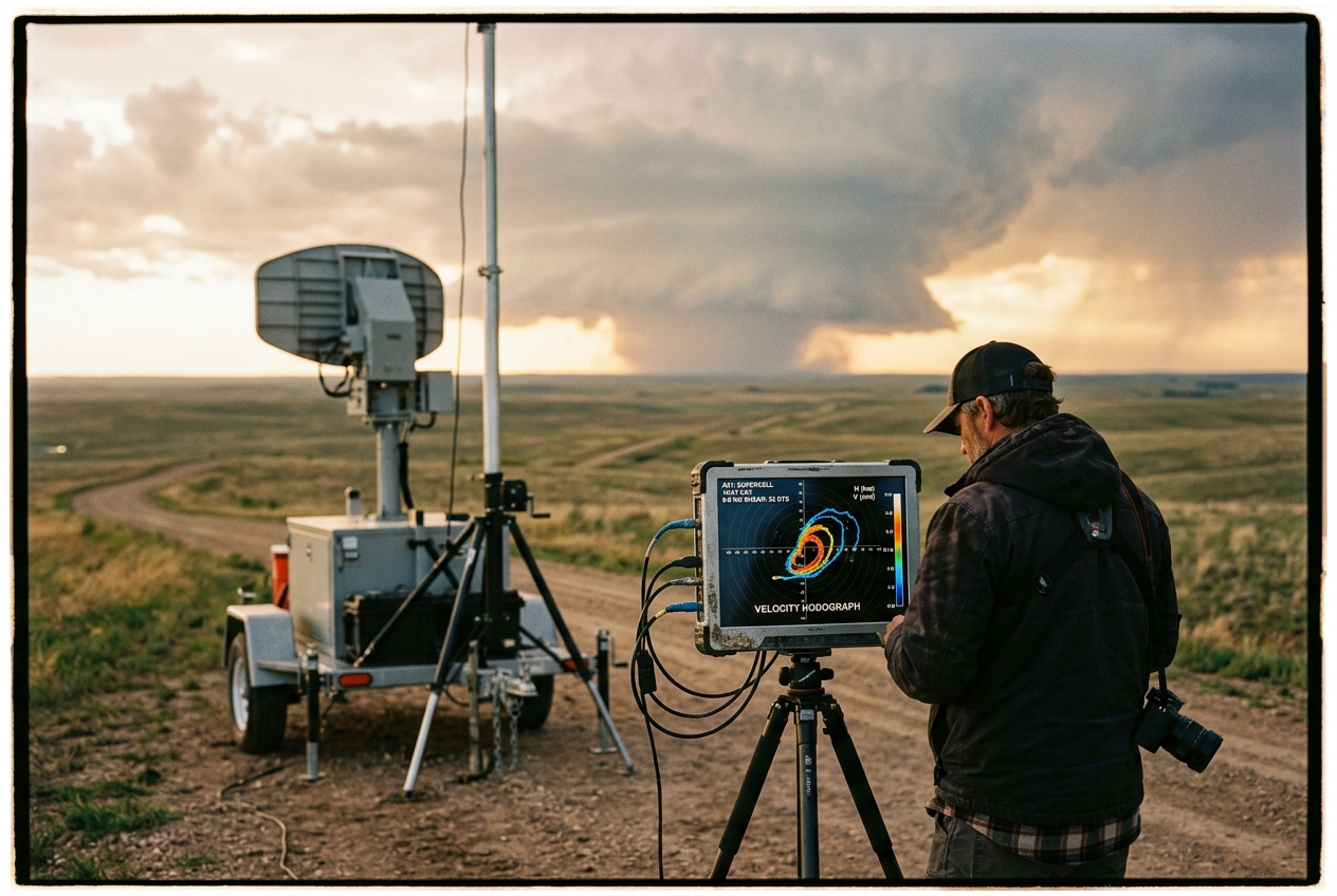
Across the open expanses of the western Great Plains in late spring, the atmosphere frequently behaves as an engine of astonishing geometric precision. An observer standing amidst the prairie grasses of western Kansas or the Oklahoma panhandle feels the midday air grow heavy and uncomfortably buoyant. The sensory cues arrive in a calculated sequence: the sharp drop in ambient barometric pressure, the sticky pull of moisture-laden boundary layer air sweeping up from the Gulf of Mexico, and the distinct, earthy tang of petrichor and nascent ozone carried on an accelerating breeze.

High above, a monolithic cumulonimbus cloud erupts, its glacial anvil spreading across the upper troposphere toward the northeast at sixty knots, following the prevailing mid-latitude jet stream. Yet, as the towering storm matures, an eerie and dramatic departure from the steering flow unfolds. While smaller rain showers and cloud fragments dutifully drift northeastward along the ambient wind, the central core of the parent thunderstorm slows, detaches from the crowd, and veers sharply to the right—tracking southeastward directly into the hot, humid low-level inflow.

To the untrained eye, this sudden lateral drift resembles a sentient navigation, a rogue giant marching against the prevailing currents. To the atmospheric physicist, it represents a deterministic consequence of three-dimensional fluid dynamics, vertical wind shear, and dynamic perturbation pressure gradients. Unlocking the logic of this deviant motion requires translating three-dimensional vertical wind profiles onto a two-dimensional polar coordinate system known as the polar hodograph, and solving the elegant vector mathematics pioneered by Matthew Bunkers.

1. What is Actually Happening? The Physics in Plain English

To understand why a severe thunderstorm turns away from the wind that created it, one must first dismantle the intuitive assumption that clouds simply drift like leaves upon a flowing river.

       UNIDIRECTIONAL SHEAR                     CYCLONIC "SICKLE" SHEAR
     (Straight-Line Hodograph)                  (Clockwise Curved Hodograph)

v (North)                                  v (North)
             |                                          |     6 km
             |    6 km                                  |    /
             |   /                                  3 km|---* 
             |  /                                     \ |  /
             | * 3 km                                  \| /
             |/                                1 km *---|' 
  -----------+----------- u (East)           -------*---+----------- u (East)
            /|                                     Sfc  |
       Sfc * |                                          |
             |                                          |
  Storm splits into equal Left &            Left-mover decays; Right-mover
  Right movers along shear axis.            deviates south/east, maximizing SRH.

The Atmosphere as a Stack of Moving Conveyor Belts

Think of the lower six kilometres of the atmosphere as a layered cake, or a series of airport conveyor belts stacked on top of one another. At the ground level, the conveyor belt may be moving relatively slowly out of the southeast at fifteen knots. Two kilometres higher, the belt accelerates and moves from the south-southwest. By the time you reach six kilometres above the surface, in the mid-tropospheric steering flow, the belt is racing out of the west at fifty knots.

This variation of wind speed and direction with height is called vertical wind shear. When air speeds change across vertical layers, friction and velocity differences set the intervening air into horizontal rotation. Picture rolling an empty cardboard tube between the palms of your hands: your lower hand moves forward slowly while your upper hand slides rapidly in another direction. The tube between them is forced to spin horizontally.

Tilting and Splitting

When an intense thunderstorm updraft—a roaring chimney of warm, buoyant air rising at fifty metres per second—punches upward through these layers, it intercepts this horizontally rolling air and bends it upward into the vertical dimension.

1. The Updraft Ingestion: As the horizontal rolls are shoved upward in the middle of the updraft, they create a pair of counter-rotating vortices on either flank of the storm: a cyclonically spinning (counter-clockwise) vortex on the right flank, and an anticyclonically spinning (clockwise) vortex on the left flank.
2. The Dynamic Pressure Deflection: As air spins rapidly within these twin vortices, the local air pressure inside them drops precipitously—just as the pressure drops in the eye of a whirlpool.
3. The Split: If the winds aloft change only in speed but not in direction (unidirectional shear), both the left and right flanks experience equal drops in dynamic pressure. The original storm splits cleanly down the middle into two distinct storms: a "left-mover" that veers to the left of the mean wind, and a "right-mover" that veers to the right.
4. The Curved Hodograph Advantage: When the wind not only increases in speed with height but also turns continuously clockwise with height (a process known as veering), dynamic vertical forces break this symmetry. A powerful vertical suction force develops exclusively on the southern (right-hand) flank of the storm, while the northern (left-hand) flank is suppressed by downward pressure. The right-hand storm is continuously sucked toward the southeast, propagating across the mean environmental flow.

2. Constructing the Polar Hodograph

To calculate these forces mathematically, atmospheric scientists map the vertical wind field obtained from rawinsondes and NOAA Doppler wind profilers onto a polar hodograph.

Mathematical Decomposition of Wind Vectors

A raw vertical wind profile provides horizontal wind velocity as a function of geometric height $z$ or pressure level $p$:

$$\mathbf{V}(z) = u(z)\hat{\mathbf{i}} + v(z)\hat{\mathbf{j}}$$

where: * $u(z) = -|\mathbf{V}(z)| \sin(\theta)$ represents the zonal velocity component (positive eastward), * $v(z) = -|\mathbf{V}(z)| \cos(\theta)$ represents the meridional velocity component (positive northward), * $\theta$ is the meteorological wind direction in degrees (the direction from which the wind blows).

   POLAR HODOGRAPH COORDINATE SYSTEM

                   North (+v)
                       |
                  30   |        * 6 km (u=20, v=15)
                       |       /
                  20   |      /
                       |  3 km
                  10   |  * 
                       | /
   --------------------+------------------- East (+u)
      -20  -10    Sfc *|    10   20   30
                       |
                       |
                   South (-v)

In a polar hodograph, the origin $(0,0)$ represents zero wind speed relative to the earth's surface. Concentric rings mark scalar wind speeds in increments of $10\text{ knots}$ or $5\text{ m s}^{-1}$.

To construct the plot: 1. Plot the tip of the surface wind vector $\mathbf{V}(0)$ as a single point at coordinates $(u_0, v_0)$. 2. Ascend incrementally through standard pressure levels ($1\text{ km}$, $2\text{ km}$, $3\text{ km}$, $6\text{ km}$), plotting each subsequent velocity tip $(u_z, v_z)$. 3. Connect these discrete points with a continuous, smoothed line curve.

The resulting line trace on the hodograph is not a physical trajectory of a parcel; it is the locus of the tips of all vertical wind vectors. The vector connecting any point $z_1$ on the hodograph to a higher point $z_2$ represents the bulk vertical shear vector ($\Delta \mathbf{V} = \mathbf{V}(z_2) - \mathbf{V}(z_1)$) across that atmospheric slice.

3. The Science: Internal Dynamics & The Bunkers Vector

The Dynamic Perturbation Pressure Equation

The physical mechanism forcing a storm to deviate from its mean steering environment is described by the diagnostic three-dimensional pressure perturbation equation derived from the Navier-Stokes equations under the anelastic approximation (Rotunno and Klemp, 1982):

$$\nabla^2 p' = -\rho_0 \left[ \left(\frac{\partial u}{\partial x}\right)^2 + \left(\frac{\partial v}{\partial y}\right)^2 + \left(\frac{\partial w}{\partial z}\right)^2 \right] - 2\rho_0 \left( \frac{\partial \mathbf{V}_h}{\partial z} \cdot \nabla_h w \right) + \rho_0 g \frac{\partial}{\partial z}\left(\frac{\theta_v'}{\bar{\theta}_v}\right)$$

Focus on the central dynamic interaction term:

$$-2\rho_0 \left( \frac{\partial \mathbf{V}_h}{\partial z} \cdot \nabla_h w \right)$$

This term governs the linear interaction between the vertical wind shear of the environment ($\frac{\partial \mathbf{V}_h}{\partial z}$) and the horizontal gradient of the storm's vertical velocity ($\nabla_h w$).

When the vertical shear vector points in a given direction, high dynamic pressure forms on the upshear flank of the updraft, while low dynamic pressure forms on the downshear flank. If the shear vector turns clockwise with height (a curved hodograph), the low-pressure anomaly shifts to the right flank of the updraft at mid-levels, creating an upward-directed Vertical Perturbation Pressure Gradient (VPPG):

$$-\frac{1}{\rho_0}\frac{\partial p'}{\partial z} > 0 \quad \text{(on the southern/right flank)}$$

This upward suction continuously induces new convective updraft growth on the right flank, forcing the storm to propagate systematically to the right of the mean environmental wind.

The Bunkers Storm Motion Algorithm

Historically, meteorologists estimated supercell motion using arbitrary empirical offsets, such as taking the mean wind and subtracting thirty degrees from the direction while reducing speed by fifteen percent. However, this failed in complex shear environments where the shear vector was oblique to the mean flow.

In 2000, Matthew J. Bunkers and his collaborators formulated an objective, Galilean-invariant technique rooted in the physical reality that the deviant dynamic force acts perpendicular to the mean vertical shear vector.

The Bunkers algorithm computes the Right-Mover ($\mathbf{c}_R$) and Left-Mover ($\mathbf{c}_L$) storm motion vectors via three discrete steps:

Step 1: Compute the Non-Dimensional Pressure-Weighted Mean Wind ($\overline{\mathbf{V}}_{0-6\text{km}}$)

The advective steering component is the pressure-weighted mean wind from the surface up to $6\text{ km}$:

$$\overline{\mathbf{V}}{0-6\text{km}} = \frac{\int{p_{\text{sfc}}}^{p_{6\text{km}}} \mathbf{V}(p)\, dp}{\int_{p_{\text{sfc}}}^{p_{6\text{km}}} dp} \approx \frac{\sum_{i=1}^{N} w_i \mathbf{V}i}{\sum{i=1}^{N} w_i}$$

where $w_i$ represents the layer thickness in pressure coordinates ($\Delta p_i$).

Step 2: Compute the Deep-Layer Shear Vector ($\mathbf{V}_{\text{shear}}$)

The bulk deep-layer vertical shear vector is defined from a surface-adjacent boundary layer ($0\text{--}500\text{ m}$) to the mid-troposphere ($5.5\text{--}6.0\text{ km}$):

$$\mathbf{V}{\text{shear}} = \overline{\mathbf{V}}{5.5-6.0\text{km}} - \overline{\mathbf{V}}{0-0.5\text{km}} = (u{\text{shear}})\hat{\mathbf{i}} + (v_{\text{shear}})\hat{\mathbf{j}}$$

Step 3: Apply the Orthogonal Deviant Deflection

The deviant propagation vector is directed perpendicular to the bulk shear vector, scaled by an empirically validated deviation speed $D \approx 7.5\text{ m s}^{-1}$ ($14.58\text{ knots}$, typically rounded to $15\text{ knots}$):

$$\mathbf{c}R = \overline{\mathbf{V}}{0-6\text{km}} + D \left( \frac{\mathbf{V}{\text{shear}} \times \hat{\mathbf{k}}}{|\mathbf{V}{\text{shear}}|} \right)$$

$$\mathbf{c}L = \overline{\mathbf{V}}{0-6\text{km}} - D \left( \frac{\mathbf{V}{\text{shear}} \times \hat{\mathbf{k}}}{|\mathbf{V}{\text{shear}}|} \right)$$

where $\hat{\mathbf{k}}$ is the vertical unit vector pointing upward.

In component form, recalling that for a two-dimensional horizontal vector $\mathbf{V}_{\text{shear}} = (u_s, v_s)$, the cross product with $\hat{\mathbf{k}}$ yields:

$$\mathbf{V}_{\text{shear}} \times \hat{\mathbf{k}} = (u_s \hat{\mathbf{i}} + v_s \hat{\mathbf{j}}) \times \hat{\mathbf{k}} = v_s \hat{\mathbf{i}} - u_s \hat{\mathbf{j}}$$

Thus, the components of the right-moving supercell velocity $\mathbf{c}_R = (u_R, v_R)$ are:

$$u_R = \bar{u} + D \frac{v_s}{\sqrt{u_s^2 + v_s^2}}$$

$$v_R = \bar{v} - D \frac{u_s}{\sqrt{u_s^2 + v_s^2}}$$

Worked Calculation: Quantifying the Rogue Vector

Let us apply the Bunkers formula to a realistic severe-weather atmospheric sounding taken ahead of a tornadic outbreak.

Given Sounding Parameters: * Pressure-Weighted Mean Wind ($0\text{--}6\text{ km}$): $\overline{\mathbf{V}}{0-6\text{km}} = 10.0\,\hat{\mathbf{i}} + 15.0\,\hat{\mathbf{j}}\text{ m s}^{-1}$ (Wind from $214^\circ$ at $18.0\text{ m s}^{-1}$) * Low-Level Wind ($0\text{--}0.5\text{ km}$ average): $\mathbf{V}{\text{low}} = 4.0\,\hat{\mathbf{i}} + 8.0\,\hat{\mathbf{j}}\text{ m s}^{-1}$ (Wind from $207^\circ$ at $8.9\text{ m s}^{-1}$) * Upper-Level Wind ($5.5\text{--}6.0\text{ km}$ average): $\mathbf{V}_{\text{high}} = 24.0\,\hat{\mathbf{i}} + 20.0\,\hat{\mathbf{j}}\text{ m s}^{-1}$ (Wind from $230^\circ$ at $31.2\text{ m s}^{-1}$) * Empirical Deviant Constant: $D = 7.5\text{ m s}^{-1}$

1. Calculate the Bulk Shear Vector ($\mathbf{V}_{\text{shear}}$)

$$\mathbf{V}{\text{shear}} = \mathbf{V}{\text{high}} - \mathbf{V}_{\text{low}} = (24.0 - 4.0)\hat{\mathbf{i}} + (20.0 - 8.0)\hat{\mathbf{j}} = 20.0\,\hat{\mathbf{i}} + 12.0\,\hat{\mathbf{j}}\text{ m s}^{-1}$$

$$|\mathbf{V}_{\text{shear}}| = \sqrt{(20.0)^2 + (12.0)^2} = \sqrt{400 + 144} = \sqrt{544} \approx 23.32\text{ m s}^{-1}$$

2. Calculate the Unit Normal Vector Components

$$n_u = \frac{v_s}{|\mathbf{V}_{\text{shear}}|} = \frac{12.0}{23.32} \approx 0.5146$$

$$n_v = -\frac{u_s}{|\mathbf{V}_{\text{shear}}|} = -\frac{20.0}{23.32} \approx -0.8576$$

3. Calculate the Right-Mover Motion Vector ($\mathbf{c}_R$)

$$u_R = \bar{u} + D(n_u) = 10.0 + 7.5(0.5146) = 10.0 + 3.86 = 13.86\text{ m s}^{-1}$$

$$v_R = \bar{v} + D(n_v) = 15.0 + 7.5(-0.8576) = 15.0 - 6.43 = 8.57\text{ m s}^{-1}$$

$$\mathbf{c}_R = 13.86\,\hat{\mathbf{i}} + 8.57\,\hat{\mathbf{j}}\text{ m s}^{-1}$$

4. Convert to Meteorological Heading and Speed

$$\text{Speed} = |\mathbf{c}_R| = \sqrt{(13.86)^2 + (8.57)^2} = \sqrt{192.10 + 73.44} = \sqrt{265.54} \approx 16.30\text{ m s}^{-1}\quad (\approx 31.7\text{ knots})$$

$$\theta_{\text{math}} = \operatorname{atan2}(v_R, u_R) = \operatorname{atan2}(8.57, 13.86) \approx 31.72^\circ$$

$$\theta_{\text{met}} = (270^\circ - \theta_{\text{math}}) \pmod{360^\circ} = 270^\circ - 31.72^\circ = 238.28^\circ \approx 238^\circ$$

CALCULATION SUMMARY: While ordinary precipitation particles and non-sheared convective showers drift toward the northeast from $214^\circ$ at $18.0\text{ m s}^{-1}$ ($35\text{ knots}$), the dynamic right-moving supercell tracks from $238^\circ$ at $16.3\text{ m s}^{-1}$ ($31.7\text{ knots}$). It moves $24^\circ$ to the right of the mean wind and slows its forward translational speed, drastically modifying its interaction with incoming low-level air parcels.

4. Storm-Relative Helicity (SRH) as a Geometric Area

Why does this rightward deviation matter so profoundly for severe weather? The answer lies in how storm motion alters the inflow of environmental vorticity.

       GEOMETRY OF STORM-RELATIVE HELICITY (SRH)

              v (North)
                  |                  * 3 km Wind Vector
                  |                 / 
                  |     Swept      /  
                  |     Area     /   
                  |   (= 1/2 SRH)
                  |     / \     /     
          1 km *--+----/---\---/       
               |  |   /     \ /        
           Sfc *  |  /       * Storm Motion Vector (c_R)
               |  | /       
   ------------+--+------------------------ u (East)
                  |

The wind entering a thunderstorm's updraft is not the ground-relative wind $\mathbf{V}(z)$, but the storm-relative wind $\mathbf{V}_{\text{sr}}(z)$:

$$\mathbf{V}_{\text{sr}}(z) = \mathbf{V}(z) - \mathbf{c}$$

Storm-Relative Helicity (SRH) quantifies the potential for convective updrafts to rotate cyclonically by measuring the transfer of streamwise vorticity from the environment into the storm. Mathematically, it is the integrated inner product of the storm-relative wind vector and the horizontal environmental vorticity vector $\boldsymbol{\omega}_h = \nabla \times \mathbf{V} = -\frac{\partial v}{\partial z}\hat{\mathbf{i}} + \frac{\partial u}{\partial z}\hat{\mathbf{j}}$:

$$\text{SRH} = \int_{0}^{h} \left[ (\mathbf{V}(z) - \mathbf{c}) \cdot \left( \hat{\mathbf{k}} \times \frac{\partial \mathbf{V}}{\partial z} \right) \right] dz = -\int_{0}^{h} \left[ (u(z) - c_u)\frac{\partial v}{\partial z} - (v(z) - c_v)\frac{\partial u}{\partial z} \right] dz$$

The Geometric Proof on the Hodograph

In polar hodograph space, this integral has an extraordinary and simple geometric identity: $\text{SRH}$ is exactly equal to twice the signed area swept out by the storm-relative wind vector as one traces the hodograph curve from the ground to height $h$.

Consider the differential area $dA$ of a triangle formed by the storm motion point $\mathbf{c} = (c_u, c_v)$ and two adjacent points on the hodograph $\mathbf{V}(z)$ and $\mathbf{V}(z + dz)$:

$$dA = \frac{1}{2} |(\mathbf{V}(z) - \mathbf{c}) \times d\mathbf{V}| = \frac{1}{2} \left[ (u(z) - c_u) dv - (v(z) - c_v) du \right]$$

Dividing by $dz$ and integrating over height yields:

$$\int_0^h dA = \frac{1}{2} \int_0^h \left[ (u - c_u)\frac{\partial v}{\partial z} - (v - c_v)\frac{\partial u}{\partial z} \right] dz = -\frac{1}{2} \text{SRH}$$

$$\text{SRH} = -2 \times \text{Area}_{\text{swept}}$$

When a storm veers to the right (from $\overline{\mathbf{V}}$ to $\mathbf{c}_R$), it shifts its reference point into the concave interior of a clockwise-curving hodograph. This rightward shift dramatically increases the swept triangular area between the storm motion point and the $0\text{--}1\text{ km}$ and $0\text{--}3\text{ km}$ hodograph segments.

A storm moving with the mean wind might experience an $0\text{--}1\text{ km SRH}$ of only $50\text{ m}^2\text{ s}^{-2}$ (insufficient for tornadogenesis). By deviating along the Bunkers vector, its $0\text{--}1\text{ km SRH}$ can surge past $250\text{--}400\text{ m}^2\text{ s}^{-2}$, converting weak environmental shear into an intense, rotating mesocyclone capable of producing violent tornadoes according to NOAA Storm Prediction Center parameters.

5. Practical Outdoor Guidance: Field Observations

Understanding hodograph kinematics allows ground observers, storm spotters, and field scientists to anticipate convective evolution directly from sensory observations and basic field instruments.

+-------------------------------------------------------------------------+
|                    FIELD OBSERVATION REFERENCE CARD                     |
+-------------------------------------------------------------------------+
| PHENOMENON               | SENSORY / INSTRUMENT CUE | KINEMATIC CAUSE   |
+--------------------------+--------------------------+-------------------+
| Backing Surface Wind     | Wind shifts from SW to   | Enlarges 0-1 km   |
|                          | SE; humidity rises       | hodograph loop;   |
|                          |                          | boosts SRH.       |
+--------------------------+--------------------------+-------------------+
| Deviant Propagation      | Radar core tracks 20-30° | VPPG suction on   |
|                          | right of anvil blow-off  | right flank via   |
|                          |                          | shear interaction.|
+--------------------------+--------------------------+-------------------+
| Anvil-Relative Inflow    | Inflow feels warm, moist | Storm-relative    |
|                          | and accelerates into the | winds ingestion of|
|                          | southern updraft base    | pure streamwise   |
|                          |                          | vorticity.        |
+--------------------------+--------------------------+-------------------+
+-------------------------------------------------------------------------+

1. What to Look for in the Sky

• Anvil vs. Base Motion Discrepancy: Observe the high, wispy cirrus shield of the thunderstorm anvil versus the low-level ragged clouds (scud) feeding into the base. If the anvil is racing northeastward while the dark, boiling base visibly expands southeastward, the storm has transitioned to a dynamic right-mover.
• The "Vault" and Inflow Bands: Look for smooth, laminar cloud bands (beaver tails or inflow bands) feeding into the southern quadrant of the storm. This confirms that the storm's deviant vector is actively drawing in pristine, un-ingested air from the warm sector.
• Striations and the "Barber Pole" Updraft: Spiral grooves etched into the updraft tower indicate that the storm is ingesting pure streamwise vorticity (rotation parallel to the inflow wind), a direct visual verification of high SRH on a curved hodograph.

2. Monitoring Field Instruments

• The Barometer: As a right-moving supercell approaches, watch for a localized, sharp barometric drop (the "mesolow") that occurs right before the sudden, violent surge of cold outflow air (the "mesohigh"). A deep dynamic low confirms intense mid-level rotation driven by vertical shear interactions.
• The Wind Vane: A critical field signature is backing surface winds. If your anemometer or wind vane shows the surface flow turning counter-clockwise over time (e.g., from south-southwest to south-southeast) while mid-level clouds advance from the west, the hodograph is rapidly expanding its low-level curvature. This is a primary warning of imminent supercell intensification.

3. A Rule of Thumb for Hikers, Sailors, and Observers

When tracking severe convection outdoors, never assume a thunderstorm will travel in the direction its upper anvil is blowing.

If you are standing with the surface wind blowing directly at your back, and you observe an isolated storm developing to your left (west or northwest) with an anvil racing across your field of view: * The Deviant Turn Hazard: The dynamic right-mover will turn toward you, moving out of the northwest toward the southeast, closing the distance far faster than linear extrapolation of upper winds would suggest. * Always calculate your escape route perpendicular to the Bunkers right-mover vector (toward the south or southwest), never downshear along the anvil's trajectory.

6. Today's Meteorological Rule of Thumb

THE HODOGRAPH SICKLE PRINCIPLE: When the vertical wind profile curves clockwise like a sickle from the ground to the mid-troposphere, the thunderstorm will reject the steering current, turn sharply right, and ingest the spin of the sheared air—transforming dynamic shear into destructive rotational power.

Authoritative References & Further Reading

• NOAA Storm Prediction Center: Sounding and Hodograph Analysis Guide
• Met Office UK: Atmospheric Shear and Cloud Dynamics
• American Meteorological Society: Glossary of Meteorology — Hodograph
• National Weather Service JetStream: Upper-Air Charts and Shear
• Bunkers, M. J., et al. (2000): Predicting Supercell Motion Using a Hodograph Technique
• Rotunno, R., and J. B. Klemp (1982): The Influence of the Shear-Induced Pressure Gradient on Thunderstorm Motion