Global Electric Circuit & Fair-Weather Potential Gradient: How Planetary Thunderstorms and Cosmic Ionization Sustain Earth's 100 V/m Ambient Field
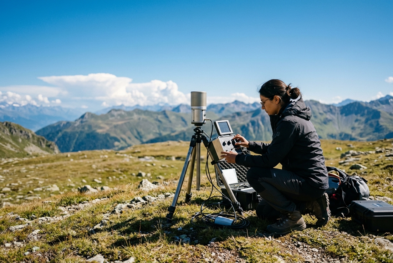
On a late August afternoon upon the open expanse of Salisbury Plain, the atmosphere undergoes a quiet, visceral metamorphosis. The air, thick with the heavy hum of late summer heat, begins to stiffen. Across the southern horizon, the sky loses its pale cerulean tint, curdling into a bruised indigo shelf of cloud. The barometer in a walker’s pack records a sharp, sudden dip, followed by a cold, sharp downdraft that rushes through the dry grass, carrying the sharp, metallic sweetness of petrichor—the smell of baked geosmin and ozone released from parched earth.
Then comes an unearthly sensation: the fine hairs upon your forearms stir and rise, standing vertically on end as though drawn upward by an unseen hand. The surrounding landscape has grown deceptively tranquil beneath the impending canopy, yet the atmosphere crackles with invisible tension. You are standing within the dielectric core of a planetary engine. Long before the first fork of cloud-to-ground lightning cleaves the horizon, an imperceptible electrical river is already coursing silently through your body, linking the soil beneath your boots to the ionized frontiers of near-space.
1. WHAT IS ACTUALLY HAPPENING: THE PLANETARY BATTERY
To understand the electrification of our atmosphere, one must abandon the intuition that air is a flawless electrical insulator. While pure dry air in a sealed laboratory offers formidable resistance, the open atmosphere behaves instead as a vast, slightly leaky spherical capacitor.
                       IONOSPHERE (+250 kV to +300 kV)
   ======================================================================
         ^                                                 |
         |  Upward Storm Currents                          |  Downward Fair-Weather
         |  (2,000 Thunderstorms)                          |  Current (J_z ~ 2 pA/m²)
         |  ~1 to 2 kA Total Dynamos                       |  Over Calm Continents/Oceans
         |                                                 v
   [ + + + + + + + ]                                [ - - - - - - - - - - ]
   [ Thunderstorms ]                                [ Fair-Weather Regime ]
   [ - - - - - - - ]                                [                     ]
         |                                                 |
         v                                                 v
   ======================================================================
                      EARTH'S SURFACE (Conductive Ground, 0 V)
Think of the Earth and its upper atmosphere as a colossal rechargeable battery coupled to an expansive global circuit—a conceptual breakthrough first proposed in the 1920s by Nobel laureate C.T.R. Wilson. In this planetary circuit: 1. The Battery Charger: At any given instant, approximately 2,000 convective storms rage simultaneously across the tropical landmasses of equatorial Africa, the Amazon basin, and the Indonesian Maritime Continent. These cumulonimbus clouds act as upward-pumping dynamos. Within their violent updrafts, collisions between graupel pellets and lighter ice crystals rip electrons away, depositing immense reservoirs of negative charge at the cloud base and lofting positive charge to the convective anvil tops. From these anvil tops, positive electric currents escape upward into the highly conductive upper atmosphere. 2. The Upper Plate: At altitudes between 60 and 100 kilometres lies the ionosphere, a rarefied sea of free electrons and ionized gas molecules bathed in solar ultraviolet radiation. The collective upward push of planetary thunderstorms pumps this layer to a staggering positive potential of +250,000 to +300,000 Volts (+250 to +300 kV) relative to the ground. 3. The Leaky Return Path: Because high-energy galactic cosmic rays and terrestrial radioactive decay continuously ionize air molecules, the atmosphere is not perfectly insulating. Across the vast, tranquil regions of the globe—the fair-weather zones where skies are clear and winds are light—this positive charge slowly and steadily trickles back down toward the negatively charged soil.
Every blade of grass, ocean wave, and human head acts as an grounded electrode receiving this quiet, persistent downward current.
2. THE SCIENCE: ION MOBILITY, CONDUCTION CURRENTS, AND POTENTIAL GRADIENTS
To quantify this invisible flow, we turn to the microscopic mechanics of atmospheric ionization and macroscopic electrodynamics.
Atmospheric Conductivity and Ion Production
The electrical conductivity of air, denoted by $\sigma(z)$, is governed by the concentration and physical mobility of trace atmospheric ions. Pure air molecules ($N_2$, $O_2$) do not conduct electricity on their own; conductivity is entirely generated by ionizing radiation: * Galactic Cosmic Rays (GCR): Relativistic protons and atomic nuclei from deep space smash into the upper and middle atmosphere, initiating hadronic and electromagnetic cascades that peak at the Pfotzer maximum (around 15 km altitude). * Terrestrial Radioactivity: Over continental crust, the radioactive decay of uranium and thorium series minerals releases gaseous radon ($^{222}\text{Rn}$) and thoron ($^{220}\text{Rn}$), emitting $\alpha$ and $\beta$ particles that ionize the lowest few hundred metres of the boundary layer.
When an air molecule loses an electron, the liberated electron attaches within nanoseconds to an oxygen molecule to form $O_2^-$. Water vapour clusters rapidly gather around these charged centers, forming hydrated cluster ions: positive "small ions" such as $H^+(H_2O)_n$ and negative small ions such as $CO_3^-(H_2O)_n$ or $NO_3^-(H_2O)_n$.
The bulk electrical conductivity $\sigma(z)$ at any altitude $z$ is the sum of the products of ion number density $n_i$, ionic mobility $\mu_i$, and the elementary electric charge $e$:
$$\sigma(z) = e \sum_i n_i(z) \, \mu_i(z) \approx e \left( n^+ \mu^+ + n^- \mu^- \right)$$
+-------------------------------------------------------------------------+
|                  WORKED PROOF: GROUND-LEVEL CONDUCTIVITY                |
+-------------------------------------------------------------------------+
| Given typical unpolluted sea-level fair-weather parameters:             |
|   - Elementary charge:         e   = 1.602 x 10^-19 C                   |
|   - Positive small ion density: n^+ = 600 cm^-3  = 6.0 x 10^8 m^-3      |
|   - Negative small ion density: n^- = 500 cm^-3  = 5.0 x 10^8 m^-3      |
|   - Positive ion mobility:     mu^+ = 1.2 x 10^-4 m^2 V^-1 s^-1         |
|   - Negative ion mobility:     mu^- = 1.4 x 10^-4 m^2 V^-1 s^-1         |
|                                                                         |
| Calculation:                                                            |
|   sigma_0 = (1.602 x 10^-19) * [ (6.0 x 10^8 * 1.2 x 10^-4)            |
|                                  + (5.0 x 10^8 * 1.4 x 10^-4) ]         |
|   sigma_0 = (1.602 x 10^-19) * [ 7.2 x 10^4 + 7.0 x 10^4 ]             |
|   sigma_0 = (1.602 x 10^-19) * [ 1.42 x 10^5 ]                          |
|   sigma_0 ≈ 2.27 x 10^-14 Siemens per metre (S/m)                       |
+-------------------------------------------------------------------------+
Because atmospheric density decreases exponentially with height while cosmic ray ionization intensifies, the mobility $\mu(z)$ and ion density $n(z)$ surge upward. Atmospheric conductivity climbs roughly exponentially with altitude:
$$\sigma(z) = \sigma_0 \exp\left(\frac{z}{s_0}\right)$$
where $s_0 \approx 5\text{ to }6\text{ km}$ represents the electrical scale height. Near the base of the ionosphere ($z \approx 60\text{ to }80\text{ km}$), conductivity is more than seven orders of magnitude greater than at the surface.
Columnar Resistance and Fair-Weather Conduction Current
If we treat a vertical atmospheric column of unit cross-sectional area ($1\text{ m}^2$) extending from the ground ($z=0$) to the ionospheric boundary ($z=z_I \approx 60\text{ km}$), its total columnar resistance $R_c$ is obtained by integrating the reciprocal of conductivity:
$$R_c = \int_0^{z_I} \frac{dz}{\sigma(z)} = \int_0^{z_I} \frac{dz}{\sigma_0 \exp(z / s_0)} \approx \frac{s_0}{\sigma_0}$$
Substituting $s_0 = 5.5 \times 10^3\text{ m}$ and $\sigma_0 = 2.27 \times 10^{-14}\text{ S/m}$ yields a columnar resistance of:
$$R_c \approx \frac{5.5 \times 10^3}{2.27 \times 10^{-14}} \approx 1.2 \times 10^{17}\ \Omega\cdot\text{m}^2$$
Remarkably, over half of this entire electrical resistance resides in the lowest 2 kilometres of the troposphere—the boundary layer where aerosol particles, dust, and humidity impede ion mobility.
With the ionosphere held at a steady potential $V_I \approx +250\text{ kV}$, Ohm's law dictates a steady vertical fair-weather conduction current density, $J_z$, directed downwards toward the Earth:
$$J_z = \frac{V_I}{R_c} \approx \frac{250 \times 10^3\text{ V}}{1.2 \times 10^{17}\ \Omega\cdot\text{m}^2} \approx 2.08 \times 10^{-12}\text{ A/m}^2 = 2.08\text{ pA/m}^2$$
Integrated over the entire fair-weather surface area of Earth ($A_{FW} \approx 5.0 \times 10^{14}\text{ m}^2$), the total global fair-weather leakage current is:
$$I_{\text{total}} = J_z \times A_{FW} \approx (2.0 \times 10^{-12}\text{ A/m}^2) \times (5.0 \times 10^{14}\text{ m}^2) \approx 1,000\text{ to }1,500\text{ Amperes}$$
A modest current of roughly one kiloampere—equivalent to the electrical draw of a few dozen domestic electric kettles—is all that flows globally to balance the planetary circuit.
The Fair-Weather Vertical Electric Field (Potential Gradient)
At any point in the atmosphere, the local vertical electric field $E_z$ is coupled to current density by Ohm's differential law: $J_z = \sigma(z) E_z(z)$.
By international convention in atmospheric electricity, the Potential Gradient (PG) is defined as the spatial derivative of electric potential with respect to height:
$$\text{PG} = \frac{dV}{dz} = -E_z = \frac{J_z}{\sigma(z)}$$
+-------------------------------------------------------------------------+
|               WORKED PROOF: SURFACE POTENTIAL GRADIENT                  |
+-------------------------------------------------------------------------+
| Given:                                                                  |
|   - Current density:      J_z      = 2.27 x 10^-12 A/m^2                |
|   - Surface conductivity: sigma_0  = 2.27 x 10^-14 S/m                  |
|                                                                         |
| Calculation:                                                            |
|   PG_0 = J_z / sigma_0                                                  |
|   PG_0 = (2.27 x 10^-12 A/m^2) / (2.27 x 10^-14 S/m)                    |
|   PG_0 = 100.0 Volts per metre (V/m)                                    |
+-------------------------------------------------------------------------+
Under clean, cloudless, fair-weather maritime conditions, the ground-level vertical potential gradient typically registers between +100 and +130 V/m.
This means that if you stand in an open, flat pasture, the electrostatic potential at the level of your nose (approx. 1.7 m above ground) is roughly +170 to +220 Volts higher than the soil upon which your shoes rest. You do not suffer an electric shock simply because your body is an electrical conductor that warps equipotential lines around your skull, and the available conduction current through such a tiny contact area is merely a few picoamperes—far beneath human sensory thresholds.
As altitude increases, because $\sigma(z)$ increases exponentially, the potential gradient drops rapidly toward zero:
$$\text{PG}(z) = \text{PG}_0 \exp\left(-\frac{z}{s_0}\right)$$
At an cruising altitude of 10 km (the flight path of commercial airliners), the potential gradient has decayed from $120\text{ V/m}$ to less than $15\text{ V/m}$.
3. THE CARNEGIE CURVE: THE PLANET'S SYNCHRONIZED HEARTBEAT
Between 1915 and 1929, the Department of Terrestrial Magnetism at the Carnegie Institution of Washington dispatched the non-magnetic research ship Carnegie across the Atlantic, Pacific, and Indian Oceans. Equipped with sensitive electrometers, scientists measured the fair-weather potential gradient thousands of miles from continental factories and mountain ranges.
   Potential Gradient (V/m)
   140 |                             __--**--__      <-- Global Peak (~19:00 UTC)
   130 |                         _--*          *--_      (Americas + Africa Storms)
   120 |                     _--*                  *
   110 |        *--__    _--*                       *--_
   100 |             *--*                               *
    90 |                                                 *--__ <-- Pacific Min (~03:00 UTC)
       +----+----+----+----+----+----+----+----+----+----+----+----+
       00   02   04   06   08   10   12   14   16   18   20   22  24 (UTC Hours)
The data revealed a phenomenon in geophysics known as the Carnegie Curve: when measured in pristine ocean air, the fair-weather electric field everywhere on Earth rises and falls in absolute synchrony according to Coordinated Universal Time (UTC / GMT), completely independent of local solar sunrise or sunset.
- The Global Trough (03:00 to 04:00 UTC): As midnight settles over Africa and the Americas, solar heating over the Pacific Ocean is minimal. With few landmasses under intense convection, planetary thunderstorm activity drops to its diurnal minimum, lowering $V_I$ and depressing the worldwide fair-weather electric field to around $90\text{ V/m}$.
- The African Ascent (12:00 to 14:00 UTC): Intense midday solar heating across the African continent and European landmass ignites widespread thunderstorm clusters, driving the circuit upward.
- The Global Crest (18:00 to 20:00 UTC): Peak late-afternoon convection over the Amazon basin and the Americas coincides with the lingering storm systems of equatorial Africa. Over 2,000 deep convective towers pump positive charge into the ionosphere simultaneously. Worldwide, the fair-weather potential gradient reaches its diurnal zenith at approximately 19:00 UTC, peaking between $130\text{ and }140\text{ V/m}$.
The Carnegie curve serves as the electrodynamic pulse of our planet's convective climate, monitored today by research programs at the World Meteorological Organization (WMO) and the National Oceanic and Atmospheric Administration (NOAA).
4. BOUNDARY LAYER PERTURBATIONS: AEROSOLS, FOG, AND SPACE CHARGE
While the open oceans mirror the clean Carnegie curve, continental measurements on land are modified by local boundary layer meteorology.
       UNPOLLUTED AIR (High Conductivity)      POLLUTED / FOGGY AIR (Low Conductivity)
       ==================================      =======================================

       Fast Small Ions (mu ~ 1.3 x 10^-4)      Aerosol Attachment: Small Ion + Nucleus
               +               -                           --> Sluggish Heavy Ion
               |               |                           (Mobility drops by 1000x!)
               v               v
          sigma_0 ≈ 2.3 x 10^-14 S/m               sigma_polluted ≈ 0.5 x 10^-14 S/m

          PG = J_z / sigma_0                      PG = J_z / sigma_polluted
             ≈ 100 V/m                               ≈ 450 V/m  (VOLTAGE SPIKE!)
The Aerosol Attachment Effect
In industrial urban basins or areas subject to agricultural burning, combustion releases millions of microscopic condensation nuclei per cubic centimetre. When highly mobile small ions ($n^{\pm}$) encounter these large aerosol particles ($Z$), they attach via diffusion:
$$n^{\pm} + Z^0 \xrightarrow{\beta} Z^{\pm}$$
The resulting large aerosol ions ($Z^{\pm}$) possess a mass thousands of times greater than small cluster ions, causing their mobility $\mu$ to drop by over three orders of magnitude (to $\sim 10^{-7}\text{ m}^2\text{V}^{-1}\text{s}^{-1}$).
Because the downward conduction current density $J_z$ is constrained by the resistance of the entire global column, $J_z$ remains roughly constant locally. Consequently, when surface conductivity $\sigma_0$ plunges due to aerosol attachment, Ohm's law forces the local potential gradient to surge:
$$\text{PG}{\text{local}} = \frac{J_z}{\sigma{\text{aerosol}}} \uparrow\uparrow$$
In dense smog or radiation fog, the surface electric field frequently spikes from its baseline $100\text{ V/m}$ to $+400\text{ to }+1,000\text{ V/m}$, turning the local boundary layer into a high-resistance choke point.
Electrode Effect and Space Charge
Near the ground, an additional complication arises: the downward electric field drives positive ions toward the surface while pulling negative ions upward. Because the solid ground cannot emit negative ions into the air, a thin zone between 1 and 10 metres above the soil becomes depleted of negative carriers. This creates a net positive space-charge layer ($\rho > 0$), which, by Gauss's Law ($\nabla \cdot \mathbf{E} = \rho / \varepsilon_0$), causes the local vertical potential gradient to increase as one approaches the ground.
5. MEASURING THE INVISIBLE: HISTORIC AND MODERN INSTRUMENTS
Atmospheric physicists rely on precision instrumentation to track these microvolt currents and kilovolt fields:
Kelvin's Water-Dropper Collector (Historic)
Devised by Lord Kelvin (William Thomson) in the 19th century, this elegant passive apparatus consists of an insulated reservoir of water with a fine nozzle protruding into the ambient air at a height $h$. As droplets detach from the nozzle tip, induction transfers electric charge between the water stream and the air until the potential of the reservoir equals the ambient atmospheric potential $V(h)$. By connecting the insulated reservoir to a calibrated quadrant electrometer, Kelvin measured the fair-weather potential gradient without requiring external power.
Modern Rotating Electric Field Mills
Modern meteorological stations operated by national forecasters such as the Met Office utilize rotating electric field mills: 1. A grounded, propeller-shaped metallic rotor spins at several thousand RPM directly above an insulated stationary stator plate. 2. As the rotor blades alternately expose and shield the stator from the atmospheric electric field, a continuous alternating displacement current is induced on the stator:
$$i(t) = \varepsilon_0 \frac{d}{dt} \left[ A_{\text{exposed}}(t) \, E_z \right]$$
- Phase-sensitive detection circuits amplify this microampere AC signal, producing a real-time, drift-free measurement of $E_z$ with millivolt-per-metre precision.
Field mills are critical safety installations at rocket launch facilities such as the Kennedy Space Center, where flight rules prohibit launches if the potential gradient exceeds $\pm 1,000\text{ V/m}$, which could trigger lightning strikes through rocket exhaust plumes.
6. PRACTICAL OUTDOOR GUIDANCE FOR THE OBSERVER
While specialized field mills provide continuous data, an observant naturalist, sailor, or mountaineer can read the electric dynamics of the atmosphere using environmental cues and standard field instruments:
+-----------------------------------------------------------------------------------+
|                     ATMOSPHERIC ELECTRICITY FIELD MATRIX                          |
+----------------------+--------------------+-------------------+-------------------+
| Weather Regime       | Expected PG (V/m)  | Instrument Signs  | Physical Sensation|
+----------------------+--------------------+-------------------+-------------------+
| Pristine Clear Sky   | +100 to +130 V/m   | Barometer steady; | Crisp, neutral air|
|                      | (Follows Carnegie) | Low aerosol count |                   |
+----------------------+--------------------+-------------------+-------------------+
| Radiation Fog / Smog | +300 to +800 V/m   | RH > 95%;         | Damp, heavy air;  |
| (Inversion Layer)    | (Positive spike)   | Wind < 2 knots    | Stagnant haze     |
+----------------------+--------------------+-------------------+-------------------+
| Developing Congestus | -500 to +2,000 V/m | Rapid baro drop;  | Sudden temperature|
| (Pre-Thunderstorm)   | (Violent swings)   | Dewpoint surge    | drop; gust front  |
+----------------------+--------------------+-------------------+-------------------+
| Active Thunderstorm  | -5,000 to          | Torrential rain;  | Hair standing;    |
| (Direct Overhead)    | +15,000 V/m        | Ozone scent       | Static on metal   |
+----------------------+--------------------+-------------------+-------------------+
What to Look for in the Sky
- Developing Cumulus Congestus: As fair-weather cumulus clouds build vertically into towering congestus plumes, watch their bases. When cloud bases darken and lower, convective charge separation begins inside the updraft. The fair-weather positive gradient at the surface under the updraft will suddenly stall, reverse sign to negative several hundred volts per metre, and then begin wild oscillations between $\pm 5,000\text{ V/m}$.
- Valley Haze and Temperature Inversions: On cold, calm mornings, look across low-lying valleys. The distinct brown line of trapped particulate pollution marks a thermal inversion layer where small ions are heavily scavenged. If you walk down into that haze layer, the local potential gradient nearly triples.
Instrument Readings to Monitor
- Aneroid Barometer: A sharp, sudden pressure drop exceeding $2\text{ hPa}$ within an hour, followed immediately by an abrupt cold gust (the thunderstorm cold pool), signals that the local atmosphere has decoupled from the fair-weather circuit and is converting into an active dynamo.
- Relative Humidity and Fog Detectors: When relative humidity hits $100\%$ in calm dawn conditions, small ion cluster radius swells from $0.8\text{ nm}$ to several micrometres as water condenses on aerosol cores. Expect ambient electrical conductivity $\sigma$ to drop by $80\%$.
Rules for Hikers, Climbers, and Sailors
- The Static Hair Warning (Immediate Evacuation): If your hair stands on end, your skin prickles, or metal gear (such as hiking poles, climbing carabiners, or a yacht's masthead rigging) begins to emit a faint buzzing or violet glow (St. Elmo's Fire), the localized potential gradient has exceeded the corona breakdown threshold of air (approx. $30\text{ kV/m}$ to $3\text{ MV/m}$ at sharp tips). Lightning attachment is imminent within seconds. Immediately crouch low on your insulating pack with feet pressed tightly together to minimize ground-stride potential, avoiding ridgelines and solitary trees.
- The 30/30 Lightning Protocol: Adopted by the Met Office and NOAA, count the seconds between seeing a flash and hearing thunder. If the interval is 30 seconds or less, the lightning is within 10 km (6 miles), indicating the local potential gradient has overwhelmed the fair-weather circuit. Seek shelter immediately, and wait 30 minutes after the last rumble before resuming outdoor activities.
TODAY'S METEOROLOGICAL RULE OF THUMB
The 100-Volt Footstep Rule: In pristine, cloudless fair weather, the invisible electrical engine of Earth's 2,000 tropical storms maintains a steady vertical potential gradient of roughly $+100\text{ Volts}$ for every metre of altitude above the soil; whenever fog, smoke, or thunderheads intrude, this delicate balance shatters—surging tenfold in stagnant smog or violently reversing sign beneath building convective storm towers.