El Niño-Southern Oscillation (ENSO) & Walker Circulation Dynamics: How Equatorial Pacific Thermal Gradients and Oceanic Kelvin Waves Drive Global Teleconnections

1. Opening Scene

Along the arid northern littoral of Peru, near the port of Paita, the air is typically defined by a cool, bracing maritime clarity. For years at a time, the prevailing southeasterly trades skim across the Humboldt Current, sweeping up chilly, nutrient-dense water from the abyssal depths and keeping the coastal plains bone-dry. The atmosphere here is usually stable, pinned down by a persistent marine inversion layer that suppresses vertical cloud development into modest stratocumulus ribbons.

Then, imperceptibly at first, the rhythm fractures.

You step outside at dawn and the sea breeze feels strangely slack, devoid of its familiar biting salt chill. By noon, the barometer on the porch—which has hovered reliably near 1014 hectopascals for months—creeps steadily downward to 1008. The skin registers an unfamiliar, suffocating tropical mugginess. Out across the western horizon, the flat marine horizon begins to boil upward. Vast, bruised towers of cumulonimbus build along the coastal cordillera, their summits flattening into immense cirrus anvils that blot out the equatorial sun.

A faint, metallic tang of ozone cuts through the dust. The sea surface, normally a brisk 18°C, is warm to the touch, resembling bathwater. Within hours, a tropical deluge strikes a desert that has not seen significant rainfall in three years, turning dry dry washes into torrents of red mud and smelling richly of petrichor and inundated clay. Thousands of miles away, on cattle stations across Queensland, Australia, the exact same geophysical event announces itself in reverse: the monsoon fails to arrive, the air dries out into a searing desiccating blast, and dust storms whip across cracked clay pans.

These twin global anomalies are not independent quirks of local meteorology. They represent the breathing cycle of the largest coupled ocean-atmosphere heat engine on Earth: the Walker Circulation and its grand, oscillatory swing known as the El Niño–Southern Oscillation (ENSO).

2. What's Actually Happening — Plain English First

To understand why a change in ocean temperature off South America can trigger droughts in Australia and disrupt winter storms over the British Isles, one must picture the tropical Pacific Ocean not as a static blue expanse, but as a colossal, fluid-filled bathtub spanning nearly half the circumference of the globe.

The Baseline Neutral Machine: The Piled-Up Ocean

Under normal, neutral conditions, the Earth’s rotation and equatorial thermal gradients sustain fierce, persistent trade winds blowing from east to west. Think of these trade winds as a household fan blowing steadily across the surface of a shallow pan of water.

As the wind pushes westward, it drags the sun-baked surface water with it across thousands of kilometers of open ocean. By the time this surface water arrives in the western Pacific near Indonesia and northern Australia, it has absorbed enormous quantities of solar radiation, pooling into an immense reservoir called the Indo-Pacific Warm Pool. Here, sea surface temperatures frequently exceed 29°C to 30°C.

Because water is piled up by the relentless push of the wind, sea level in the western Pacific is actually about 50 centimeters higher than it is in the eastern Pacific off Ecuador.

In the east, near South America, the surface water dragged away to the west must be replaced. It is drawn from the cold ocean interior—a process known as equatorial upwelling. A sharp thermal boundary beneath the ocean surface, known as the thermocline (the dividing zone separating the sun-warmed upper layer from the frigid abyssal ocean), is pulled upward toward the surface in the east, sitting just 30 to 50 meters deep. In the west, the thermocline is driven down to depths of 150 to 200 meters.

This oceanic asymmetry creates an atmospheric loop named the Walker cell in honour of Sir Gilbert Walker: 1. Ascent in the West: Over the warm pool, heated water warms the overlying air, which becomes buoyant, moist, and rises in towering convective storms. 2. High-Altitude Transport: Reaching the upper troposphere (around 12–15 km altitude), the dried air travels eastward. 3. Descent in the East: Cooling by radiation, the air becomes dense and sinks over the cold eastern Pacific waters, creating high surface atmospheric pressure and clear, dry skies. 4. Surface Return: The air completes the circuit by blowing back west as the easterly trade winds.

The Oscillation: El Niño and La Niña

The system does not stay locked in this equilibrium. It acts like a giant atmospheric-oceanic teeterboard.

• El Niño (The Warm Phase): If the trade winds slacken even slightly, the massive pile of warm western water sloshes back downhill toward the central and eastern Pacific. As the warm water moves east, the locus of atmospheric convection travels with it. The eastern Pacific warms dramatically, the cold upwelling is suppressed, the thermocline flattens, and the Walker circulation breaks down or fragments into multiple weaker cells.
• La Niña (The Supercharged Cold Phase): Conversely, when the trade winds blow with anomalous ferocity, they pile even more warm water into the far west, pull the eastern thermocline even closer to the surface, and supercharge the cold tongue. The Walker circulation spins up into overdrive.

3. The Science (for those who want to go deeper)

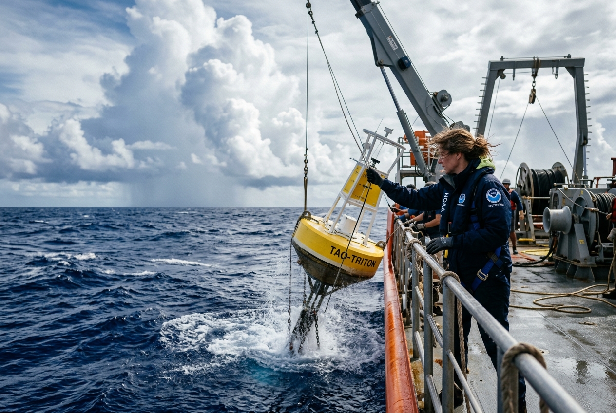
To transition from conceptual intuition to geophysical fluid dynamics, we must examine the coupled oceanic-atmospheric feedbacks that govern this vast system, tracked continuously by agencies like the National Oceanic and Atmospheric Administration (NOAA) and the Met Office.

The Bjerknes Positive Feedback Mechanism

The self-amplifying nature of ENSO was first rigorously synthesized by meteorologist Jacob Bjerknes in 1969. Bjerknes recognized that the ocean and atmosphere over the equatorial Pacific do not merely interact; they form a tightly coupled positive feedback loop:

$$\text{Trade Wind Weakening} \longrightarrow \text{Eastward Warm Water Advection} \longrightarrow \text{Zonal SST Gradient Reduction} \longrightarrow \text{Zonal Pressure Gradient Collapse} \longrightarrow \text{Further Trade Wind Weakening}$$

When an initial westerly wind burst occurs over the western equatorial Pacific, it generates an internal oceanic wave known as a downwelling Equatorial Kelvin Wave. Because the Coriolis parameter $f = 2\Omega\sin\phi$ vanishes at the equator ($\phi = 0$), the equator behaves as a natural dynamic waveguide. These Kelvin waves propagate eastward across the basin at phase speeds of roughly 2 to 3 meters per second:

$$c = \sqrt{g' H}$$

where $g' = g \frac{\Delta \rho}{\rho_0}$ is the reduced gravity (accounting for the slight density difference across the thermocline, typically $\approx 0.02\text{ to }0.03\text{ m/s}^2$) and $H$ is the equivalent mixed layer depth ($\approx 100\text{ to }150\text{ m}$).

Upon reaching the South American coast, the downwelling Kelvin wave depresses the thermocline, preventing cold water from reaching the surface layer. This warms the eastern Pacific sea surface temperature ($SST$). The warmer ocean decreases the sea level pressure in the east, which collapses the east-west atmospheric pressure gradient, causing the trade winds to slacken further. This circular positive feedback drives the system into a full-blown El Niño event.

Key Metric 1: The Southern Oscillation Index (SOI)

The atmospheric component of ENSO is quantified by measuring the normalized sea level pressure difference between Tahiti (representing the eastern Pacific subtropical high) and Darwin, Australia (representing the western Pacific equatorial low).

What the Equation Predicts

The Southern Oscillation Index (SOI) measures how vigorously the atmospheric Walker cell is pumping. A strongly negative value signals that eastern Pacific pressures have crashed while western pressures have spiked—the classical signature of El Niño. A strongly positive value indicates an intense pressure gradient driving hyperactive trade winds—the signature of La Niña.

The Mathematical Formulation

The Australian Bureau of Meteorology calculates the standardized Troup SOI as follows:

$$SOI = 10 \times \left( \frac{P_{\text{diff}} - \overline{P_{\text{diff}}}}{\sigma(P_{\text{diff}})} \right)$$

Where: * $P_{\text{diff}} = P_{\text{Tahiti}} - P_{\text{Darwin}}$ (the monthly mean sea-level pressure difference). * $\overline{P_{\text{diff}}}$ is the long-term climatological mean of that pressure difference for that specific calendar month. * $\sigma(P_{\text{diff}})$ is the long-term standard deviation of that pressure difference for that calendar month. * The factor of $10$ is a conventional scaling multiplier to yield integer-friendly values.

Worked Example with Realistic Geophysical Numbers

Let us calculate the SOI during a pronounced El Niño event for the month of November:

1. Historical Climatological Baselines (November): * Long-term average pressure difference: $\overline{P_{\text{diff}}} = +2.8\text{ hPa}$ (Tahiti typically higher than Darwin). * Long-term standard deviation: $\sigma(P_{\text{diff}}) = 1.6\text{ hPa}$.

2. Observed Monthly Station Pressures: * Measured Tahiti Sea Level Pressure: $P_{\text{Tahiti}} = 1010.2\text{ hPa}$ (anomalously low by $-2.0\text{ hPa}$). * Measured Darwin Sea Level Pressure: $P_{\text{Darwin}} = 1011.0\text{ hPa}$ (anomalously high by $+1.4\text{ hPa}$).

3. Computation: * Calculate current difference: $$P_{\text{diff}} = 1010.2 - 1011.0 = -0.8\text{ hPa}$$ * Calculate anomaly relative to long-term mean: $$\Delta P = P_{\text{diff}} - \overline{P_{\text{diff}}} = -0.8 - (+2.8) = -3.6\text{ hPa}$$ * Standardize and scale: $$SOI = 10 \times \left( \frac{-3.6}{1.6} \right) = 10 \times (-2.25) = \mathbf{-22.5}$$

Key Metric 2: Equatorial Ocean-Atmosphere Balance & Thermocline Tilt

In the steady-state equatorial ocean, the zonal (east-west) slope of the thermocline is held in balance by the wind stress exerted by the trade winds on the surface layer.

What the Equation Predicts

This reduced-gravity equilibrium equation predicts how much the thermocline depth must tilt across the Pacific basin ($L \approx 15,000\text{ km}$) to balance the mechanical drag of the easterly trade winds. When wind stress $\tau_x$ drops to near zero, the internal thermocline slope must collapse toward horizontal.

The Mathematical Formulation

$$g' \frac{\partial h}{\partial x} = \frac{\tau_x}{\rho_0 H}$$

Rearranging to solve for the total thermocline depth difference across the basin ($\Delta h = h_{\text{west}} - h_{\text{east}}$):

$$\Delta h = \frac{\tau_x \cdot L}{\rho_0 g' H}$$

Where: * $\tau_x$ = Zonal surface wind stress exerted by the atmosphere ($\text{N/m}^2$, negative for easterly winds). * $L$ = Basin width ($\approx 1.5 \times 10^7\text{ m}$). * $\rho_0$ = Mean sea water density ($\approx 1025\text{ kg/m}^3$). * $g'$ = Reduced gravity across the pycnocline ($\approx 0.025\text{ m/s}^2$). * $H$ = Mean depth of the upper mixed layer ($\approx 100\text{ m}$).

Worked Example

Consider a transition from a standard neutral state to a collapsed El Niño state:

1. Neutral Easterly Trade Wind Case: * Assume steady easterly wind stress $\tau_x = -0.05\text{ N/m}^2$. * Denominator product: $\rho_0 g' H = (1025) \times (0.025) \times (100) \approx 2562.5\text{ N/m}^2$. * Total thermocline depth differential: $$\Delta h = \frac{0.05 \times (1.5 \times 10^7)}{2562.5} = \frac{750,000}{2562.5} \approx \mathbf{292.7\text{ m}}$$ * The thermocline sits $\approx 200\text{ m}$ deep in the western Pacific and shelves steeply up to $\approx 30\text{ m}$ in the east.

2. El Niño Wind Slackening Case: * The trade winds collapse, reducing wind stress to $\tau_x = -0.01\text{ N/m}^2$. * The balanced depth differential drops to: $$\Delta h = \frac{0.01 \times (1.5 \times 10^7)}{2562.5} \approx \mathbf{58.5\text{ m}}$$

Atmospheric Teleconnections: The Planetary Wave Train

The collapse of the Walker circulation does not stay confined to the tropics. Tropical convection acts as a massive thermal chimney for the entire planet. When the primary chimney shifts $6,000\text{ km}$ eastward into the central-eastern Pacific, it forces massive divergent air outflows in the upper troposphere (near $200\text{ hPa}$).

This anomaly acts as an obstacle to the mid-latitude jet stream, exciting planetary-scale Rossby wave trains that propagate poleward and eastward.

In the Northern Hemisphere, this manifests as the Pacific-North American (PNA) pattern: 1. Deepening of the Aleutian Low in the North Pacific. 2. Amplification of a high-pressure ridge over northwestern North America (bringing unseasonably warm winters to Canada and Alaska). 3. Displacement of the Pacific jet stream southward, funneling atmospheric rivers and torrential rains across southern California and the Gulf Coast.

In Europe, the downstream teleconnection alters the North Atlantic Oscillation (NAO), often preconditioning the late winter for split polar vortex events or protracted blocking highs, as monitored by the World Meteorological Organization (WMO).

4. Practical Outdoor Guidance

While ENSO operates on seasonal-to-interannual scales, an astute outdoors person, sailor, or gardener can observe its real-time atmospheric fingerprints and adapt their planning accordingly.

What to Look for in the Sky

• Subtropical Jet Stream Cloud Filaments: Look for persistent bands of high-altitude cirrus moving rapidly from the southwest toward the northeast in winter. During El Niño years, the subtropical jet stream is unusually strong and energized across the southern latitudes of North America and Europe.
• Suppressed Convective Depth in Tropics/Subtropics: In regions like Australasia during an El Niño, summer cumulus clouds will appear stunted and sheared off, failing to build into towering storm clouds due to wide-scale atmospheric subsidence (sinking air).

Instrument Readings to Watch

• The Barometer: Keep a running log of monthly sea level pressure anomalies. A consistent positive offset of $+2\text{ to }+4\text{ hPa}$ in the western Pacific/Australasia indicates the descending branch of a broken Walker cell, heralding protracted drought conditions.
• Ocean Surface Temperature Gauges: For coastal mariners, logging sea surface temperature ($SST$) provides direct evidence of thermocline behavior. Rapid warming along the eastern boundaries of ocean basins (e.g., eastern Pacific or eastern Atlantic) accompanied by water clarity changes indicates suppressed nutrient upwelling.

Strategic Rules of Thumb for Practitioners

• For the Sailor: When crossing equatorial regions during El Niño phases, anticipate the traditional Intertropical Convergence Zone (ITCZ) "doldrums" to shift south and broaden longitudinally. Trade winds in the normal $10^\circ\text{N}-15^\circ\text{N}$ belt will frequently become variable or reverse to westerly.
• For the Grower and Agronomist: Track the quarterly forecasts from authoritative climate portals like NOAA Climate.gov. If a transition to El Niño with a high Oceanic Niño Index ($ONI > +1.5^\circ\text{C}$) is declared in early spring, prepare for hot, dry conditions in eastern Australia and southern Africa, but prepare soil drainage systems for excess rainfall across the southern United States and coastal South America.

5. Today's Meteorological Rule of Thumb

Whenever you observe a prolonged shift in your regional seasonal weather patterns, remember that the atmosphere is not acting in isolation. It is dancing in rhythm with the sloshing of warm water across the vast Pacific basin, tied across thousands of miles by the unseen, planetary gears of the Walker Circulation.