Corfidi Vectors & Mesoscale Convective System Propagation: How Inflow Kinematics and Cell Vector Addition Forecast Back-Building Deluges and Fast-Moving Derechos
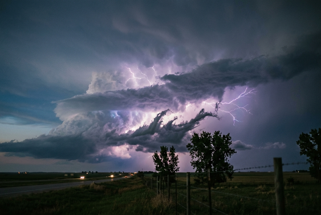
How the delicate kinematic geometry of Kevin Corfidi solved meteorology's greatest forecasting paradox—distinguishing the stalling deluge of flash floods from the supersonic frenzy of derechos.
1. Atmospheric Portents: The Stagnant Valley and the Racing Wind
On a sweltering midsummer evening in the lee of a mountain range, the atmosphere hangs with the oppressive weight of a wet wool blanket. The ambient temperature hovers near 33°C, yet the air feels considerably hotter; the dew point has climbed past 22°C, saturating the boundary layer with invisible water vapour. The air is so stagnant that the leaves on the poplars refuse to stir. Sweat refuses to evaporate from bare skin, condensing into steady rivulets instead. There is a palpable, electrostatic tension in the environment—a sharp metallic tang in the nostrils, reminiscent of hot electrical wiring mixed with the earthy perfume of dry topsoil awaiting rain.
Look toward the western horizon. What began as innocent, cauliflower-like cumulus congestus towers at mid-afternoon has metastasised into an ominous, monolithic anvil. The cloud base is an bruised underbelly of charcoal and slate, boiling upwards through the troposphere to pierce the tropopause at nearly fifteen kilometres. High above, the setting sun illuminates the crisp, glaciated fibrous plume of cirrus spreading downwind. At the surface, however, the barometer begins a steady, rhythmic descent.
                                    STORM CLUSTERS: TWO OPPOSING FATES

   BACK-BUILDING DELUGE (Quasi-Stationary)           FORWARD-PROPAGATING DERECHO (Progressive)

        Steering Flow (V_cloud) --->                      Steering Flow (V_cloud) --->
      ==============================                    ==============================
      [Cell 3] <- [Cell 2] <- [Cell 1]                  [Cell 1] -> [Cell 2] -> [Cell 3] ===>>
      (New updraft)   (Mature)  (Rainout)               (Rainout)   (Mature)  (Bow Apex) (120 km/h)
      ------------------------------                    ---------------------------------------
      <--- Inflow Jet (V_LLJ)                           <--- Inflow Jet (V_LLJ)
      Result: Anchors over single basin (300 mm)        Result: Accelerating cold-pool bow wave
Suddenly, the suffocating calm fractures. A cool draught—smelling sharply of ozone and pulverized rain—washes across the landscape. The barometric trace on a home weather station abruptly spikes upward by three millibars in a matter of seconds, registering the sudden arrival of an evaporatively cooled mesohigh. Yet here lies the profound meteorological riddle that has humbled forecasters for generations: what will this storm complex do next?
Under virtually identical synoptic jet stream patterns, two superficially indistinguishable storm clusters can produce diametrically opposed human catastrophes. In one county, the storm system anchors itself over a single mountainous drainage basin for five unrelenting hours. The sky unleashes a relentless, stationary bombardment of cloudbursts that drops 300 millimetres of rainfall, transforming placid creeks into catastrophic torrents of mud and debris. In a neighbouring state, an identical cluster reorganises into a forward-surging, bow-shaped arc of kinetic fury, tearing across three time zones at 110 kilometres per hour, levelling forests and severing high-voltage electrical grids over an eight-hundred-kilometre swath.
To understand why one storm cluster commits geographical suicide by lingering until it drowns the landscape while another accelerates into a supersonic gale, atmospheric scientists must look past the individual thunderstorm cell and examine the elegant vector kinematics of the Mesoscale Convective System (MCS).
2. What Is Actually Happening: Uncoupling the Cell from the System
To unlock this puzzle, one must first dismantle a widespread misconception: a storm system is not a single, monolithic entity that simply drifts with the prevailing wind like a leaf upon a stream. Rather, an MCS is a living, self-replicating ecological collective of convective cells, where parent storms continuously birth child storms along their outflow margins.
Think of the troposphere as an immense, multi-tiered conveyor belt. When an individual thunderstorm updraft forms, it draws warm, buoyant air upward, converts water vapour into liquid droplets and hail, and eventually collapses under the sheer weight of its accumulated precipitation. This collapsing downdraft hits the ground and spreads out laterally in all directions as a dense, chilly bubble of air known as a cold pool.
                           THE DUAL NATURE OF STORM MOTION

                  ===================================================
                  SYSTEM VELOCITY (V_system) = ADVECTION + PROPAGATION
                  ===================================================

                       [ Individual Cell Advection ]
                                 (V_cloud)
                     Steered by 850-300 hPa Mean Winds
                                     +
                       [ New Updraft Propagation ]
                                 (V_prop)
                     Forced by Cold-Pool & Low-Level Jet
                                     =
                       [ Resultant System Vector ]
                                (V_system)
Here we encounter the fundamental distinction in radar meteorology:
- Advection ($\mathbf{V}{\text{cell}}$ or $\mathbf{V}{\text{cloud}}$): The passive translation of existing individual storm cells carried along by the deep, mid-tropospheric steering currents (the mean wind between roughly 1.5 km and 9 km above sea level).
- Propagation ($\mathbf{V}_{\text{prop}}$): The systematic birth and positioning of new updrafts along the leading edge of the storm's expanding cold pool, where the dense outflow acts as a miniature, razor-sharp cold front plowing into the surrounding tropical air mass.
The Locomotive and Treadmill Analogies
To visualise how advection and propagation interact, imagine a passenger walking briskly down the aisle of a passenger train. The train is cruising eastward at 50 km/h; the passenger walks toward the dining car at 5 km/h. To an observer standing on the railway platform, the passenger moves eastward at 55 km/h if walking toward the front, but at 45 km/h if walking toward the rear.
Now, refine this analogy into what atmospheric scientists call the treadmill effect or the train-car effect. Imagine a long fitness treadmill whose belt is running briskly from west to east at 40 km/h (representing the mid-level steering winds carrying individual cells downwind). If a runner stands on that treadmill and sprints toward the west at precisely 40 km/h (representing the ignition of new convective cells upwind), their net physical position relative to the room remains perfectly stationary.
                               THE TREADMILL EFFECT

    Steering Winds (V_cloud) --->  [Cell 3 (Decaying)] ---> Eastward Advection
    -------------------------------------------------------------------------
    Westward Inflow (V_LLJ)  <---  [Cell 1 (New Born)] <--- Upwind Propagation
    -------------------------------------------------------------------------
                     NET POSITION: ZERO GROUND DISPLACEMENT (DELUGE)
Each individual runner (cell) is born at the front of the deck, gets swept backward toward the rear as they tire and rain out, but a fresh runner instantly steps onto the front of the deck to replace them. To an observer on the ground, the rain never stops falling over that single geographic coordinate.
Conversely, if the runner turns around and sprints in the same direction as the moving belt, their forward speed combines with the belt's velocity. The runner hurtles forward at blistering speed. In atmospheric physics, when the cold pool pushes aggressively forward and the inflow of buoyant fuel continuously builds new cells along its advancing downwind flank, the entire convective complex accelerates into a freight-train gale known as a derecho.
3. The Science: Kevin Corfidi's Kinematic Vector Mechanics
In the late 1990s and early 2000s, Kevin Corfidi, a lead forecaster at the NOAA Storm Prediction Center, transformed severe convective forecasting by developing an operational vector-addition framework. Corfidi recognized that system-scale storm motion could be accurately diagnosed by decomposing the atmosphere into two primary kinematic components:
- The Mean Cloud-Layer Wind ($\mathbf{V}_{\text{cloud}}$): The density-weighted mean wind vector spanning the 850 hPa to 300 hPa pressure levels (roughly 1.5 km to 9 km altitude). This vector dictates the passive advection speed and direction of individual radar echoes: $$\mathbf{V}{\text{cell}} \approx \mathbf{V}{\text{cloud}}$$
- The Low-Level Jet Vector ($\mathbf{V}_{\text{LLJ}}$): The wind vector within the lowest boundary layer (typically measured at the 850 hPa level, approximately 1.5 km above ground). This represents the high-octane conduit delivering warm, moist, high-equivalent-potential-temperature ($\theta_e$) air directly into the storm's gust front.
Because new convective cells are preferentially triggered where this low-level moisture inflow impinges directly upon the storm's dense, evaporatively cooled gust front, the propagation vector ($\mathbf{V}{\text{prop}}$) points in the exact opposite direction of the Low-Level Jet: $$\mathbf{V}{\text{prop}} = -\mathbf{V}_{\text{LLJ}}$$
By performing vector addition on a meteorological hodograph—a polar coordinate graph displaying wind speed and direction across vertical atmospheric layers—forecasters can calculate two critical vectors: the Upwind (Back-Building) Corfidi Vector and the Downwind (Forward-Propagating) Corfidi Vector.
                            HODOGRAPH VECTOR ADDITION

                       North (0°)
                           ^
                           |            . (V_cloud: 240° / 35 kt)
                           |           /
                           |          /
       West (270°) <-------+-------> / --------> East (90°)
                           |        /
       (V_LLJ: 180° / 30 kt)|       /
              |            |      /
              v            |     /
             [*]           |    /
                           v   /
                       South (180°)

      Back-Building Vector (V_back) = V_cloud - V_LLJ
      Forward Vector (V_forward)    = V_cloud + V_LLJ (modified by cold pool)
Mathematical Proof 1: The Back-Building (Quasi-Stationary) Vector
The Upwind Corfidi Vector ($\mathbf{V}_{\text{back}}$) models storm systems where regeneration occurs along the upwind or trailing flank of the cold pool. It defines the net velocity of the mesoscale convective system as the vector sum of cell advection and upwind propagation:
$$\mathbf{V}{\text{back}} = \mathbf{V}{\text{cell}} + \mathbf{V}{\text{prop}} = \mathbf{V}{\text{cloud}} - \mathbf{V}_{\text{LLJ}}$$
Step-by-Step Worked Example
Consider a classic summer flash-flood sounding analysed by the Met Office or NOAA National Severe Storms Laboratory. We decompose the meteorological wind vectors into standard Cartesian $(u, v)$ zonal (west-to-east) and meridional (south-to-north) components, where: $$u = -V \cdot \sin(\theta), \quad v = -V \cdot \cos(\theta)$$ (with $\theta$ representing the direction from which the wind blows, in degrees).
-
Mean Cloud-Layer Wind ($\mathbf{V}_{\text{cloud}}$): Unidirectional south-westerly steering flow blowing from $225^\circ$ at a speed of $28.3\text{ knots}$ ($14.5\text{ m/s}$). $$u_{\text{cloud}} = -28.3 \cdot \sin(225^\circ) = -28.3 \cdot (-0.7071) = +20.0\text{ kt}$$ $$v_{\text{cloud}} = -28.3 \cdot \cos(225^\circ) = -28.3 \cdot (-0.7071) = +20.0\text{ kt}$$ $$\mathbf{V}_{\text{cloud}} = (20.0, 20.0)\text{ kt}$$
-
Low-Level Jet ($\mathbf{V}_{\text{LLJ}}$): A potent nocturnal inflow jet blowing from the south-southwest at $207^\circ$ at a speed of $22.4\text{ knots}$ ($11.5\text{ m/s}$). $$u_{\text{LLJ}} = -22.4 \cdot \sin(207^\circ) = -22.4 \cdot (-0.4540) = +10.17\text{ kt}$$ $$v_{\text{LLJ}} = -22.4 \cdot \cos(207^\circ) = -22.4 \cdot (-0.8910) = +19.96\text{ kt}$$ $$\mathbf{V}_{\text{LLJ}} \approx (10.2, 20.0)\text{ kt}$$
Now, compute the resultant Back-Building Corfidi Vector ($\mathbf{V}{\text{back}}$): $$\mathbf{V}{\text{back}} = \mathbf{V}{\text{cloud}} - \mathbf{V}{\text{LLJ}}$$ $$u_{\text{back}} = u_{\text{cloud}} - u_{\text{LLJ}} = 20.0 - 10.2 = +9.8\text{ kt}$$ $$v_{\text{back}} = v_{\text{cloud}} - v_{\text{LLJ}} = 20.0 - 20.0 = 0.0\text{ kt}$$
Calculate the magnitude ($|\mathbf{V}{\text{back}}|$) and resultant direction ($\theta{\text{back}}$): $$|\mathbf{V}{\text{back}}| = \sqrt{(9.8)^2 + (0.0)^2} = 9.8\text{ knots}\; (\approx 18.1\text{ km/h})$$ $$\theta{\text{back}} = 270^\circ\; (\text{drifting slowly due eastward})$$
+-----------------------------------------------------------------------------+
| CALLOUT: THE ANATOMY OF A DELUGE                                            |
| While individual convective cells race northeastward at nearly 30 knots     |
| (55 km/h), new cells erupt on the southwestern flank at an equal and        |
| opposite rate. The aggregate storm complex crawls eastward at under 10      |
| knots. Over a single mountain watershed, five distinct supercells pass      |
| directly overhead in succession, unleashing catastrophic flash flooding.    |
+-----------------------------------------------------------------------------+
Mathematical Proof 2: The Forward-Propagating (Derecho) Vector
When an expansive, cold, dense downdraft pools beneath a cluster of storms, hydrostatic pressure within the cold pool rises, forming a mesoscale high-pressure dome. The horizontal pressure gradient between this cold pool and the pristine ambient environment drives a ferocious density current forward.
If low-level environmental vertical wind shear is sufficiently balanced by the cold pool's vorticity (governed by the famous Rotunno-Klemp-Weisman (RKW) theory), the system transitions into a forward-propagating convective system. New cells are violently forced upward along the downwind leading edge.
Under these conditions, system-scale velocity is determined by adding the propagation vector in the direction of the mean steering flow:
$$\mathbf{V}{\text{forward}} = \mathbf{V}{\text{cell}} - \mathbf{V}{\text{prop}} = \mathbf{V}{\text{cloud}} + \mathbf{V}_{\text{LLJ}}$$
Step-by-Step Worked Example
Let us examine the atmospheric profile typical of a major continental derecho:
-
Mean Cloud-Layer Wind ($\mathbf{V}_{\text{cloud}}$): Strong westerly mid-level flow blowing from $270^\circ$ at $45.0\text{ knots}$ ($23.1\text{ m/s}$). $$u_{\text{cloud}} = -45.0 \cdot \sin(270^\circ) = +45.0\text{ kt}, \quad v_{\text{cloud}} = 0.0\text{ kt}$$ $$\mathbf{V}_{\text{cloud}} = (45.0, 0.0)\text{ kt}$$
-
Low-Level Jet ($\mathbf{V}_{\text{LLJ}}$): A robust boundary-layer feeding jet blowing from the south-west at $225^\circ$ at $35.0\text{ knots}$ ($18.0\text{ m/s}$). $$u_{\text{LLJ}} = -35.0 \cdot \sin(225^\circ) = +24.75\text{ kt}$$ $$v_{\text{LLJ}} = -35.0 \cdot \cos(225^\circ) = +24.75\text{ kt}$$ $$\mathbf{V}_{\text{LLJ}} = (24.75, 24.75)\text{ kt}$$
Now calculate the Forward-Propagating Corfidi Vector ($\mathbf{V}{\text{forward}}$): $$\mathbf{V}{\text{forward}} = \mathbf{V}{\text{cloud}} + \mathbf{V}{\text{LLJ}}$$ $$u_{\text{fwd}} = u_{\text{cloud}} + u_{\text{LLJ}} = 45.0 + 24.75 = +69.75\text{ kt}$$ $$v_{\text{fwd}} = v_{\text{cloud}} + v_{\text{LLJ}} = 0.0 + 24.75 = +24.75\text{ kt}$$
Calculate the net forward speed and propagation bearing: $$|\mathbf{V}{\text{forward}}| = \sqrt{(69.75)^2 + (24.75)^2} = \sqrt{4865.06 + 612.56} = \sqrt{5477.62} \approx 74.01\text{ knots}\; (137.1\text{ km/h})$$ $$\theta{\text{fwd}} = 270^\circ - \arctan\left(\frac{24.75}{69.75}\right) = 270^\circ - 19.5^\circ = 250.5^\circ\; (\text{moving toward } 070.5^\circ \text{ / ENE})$$
+-----------------------------------------------------------------------------+
| CALLOUT: THE SUPER DERECHO SPRINT                                           |
| The individual cells inside this complex move at 45 knots, but the entire   |
| convective bow echo races across the landscape at an astonishing 74 knots   |
| (137 km/h). The storm outruns ordinary synoptic weather fronts, producing   |
| continuous straight-line hurricane-force wind gusts along its path.         |
+-----------------------------------------------------------------------------+
4. Historical Case Benchmarks: Two Faces of Mesoscale Fury
To appreciate the real-world operational power of Corfidi vector analysis, we can examine two historical catastrophes that forever altered the science of hydrometeorology and severe storm forecasting.
                           HISTORICAL BENCHMARKS COMPARISON

   METRIC                   1976 BIG THOMPSON CANYON        2012 NORTH AMERICAN DERECHO
   ====================================================================================
   Primary Dynamic Mode     Back-Building / Quasi-Stationary Progressive / Bow Echo
   Steering Flow (V_cloud)  Weak South-Southwest (15 kt)     Strong West-Northwest (50 kt)
   Low-Level Jet (V_LLJ)    Potent East-Southeast (35 kt)    Moist South-Southwest (40 kt)
   Vector Interaction       V_cell + V_prop ≈ 0 kt (Stall)   V_cell + V_prop ≈ 70 kt (Surge)
   Peak Impact              300 mm rain in 4 hours           140 km/h wind gusts over 1,100 km
   Human / Economic Toll    144 fatalities; canyon devastated 28 fatalities; $2.9B USD damage
The 1976 Big Thompson Canyon Disaster: The Stalled Killer
On the evening of July 31, 1976, in the rugged terrain of Larimer County, Colorado, an event unfolded that remains a benchmark in the annals of the World Meteorological Organization. A massive, moisture-laden air mass with precipitable water values exceeding 35 mm (anomalously high for the semi-arid Rockies) was pushed westward across the Great Plains.
                               BIG THOMPSON CANYON KINEMATICS

                               [ Rocky Mountain Escarpment ]
                                      |         ^
   Easterly Inflow Jet (V_LLJ)        |         |  Individual Cell Advection
   (30-35 kt Upslope) ===============>|         |  (V_cloud: 15 kt Southerly)
                                      |         |
                                      |   [Stagnant Anchor Point]
                                      |   Continuous cell regeneration
                                      |   cancels downstream translation
The upper-level steering winds ($\mathbf{V}{\text{cloud}}$) were extremely weak and oriented south-to-north at approximately 15 knots. Simultaneously, a fierce, low-level easterly inflow jet ($\mathbf{V}{\text{LLJ}}$) of 30 to 35 knots rammed into the mountain escarpment.
When forecasters subsequently applied the Back-Building Corfidi equation: $$\mathbf{V}{\text{back}} = \mathbf{V}{\text{cloud}} - \mathbf{V}_{\text{LLJ}}$$
The easterly moisture vector precisely counteracted the weak steering currents at the ridge line. The storm system anchored itself directly over the mouth of the Big Thompson Canyon. As individual convective cells matured and drifted north, new updrafts were explosively triggered in the exact same upstream location by the relentless easterly jet slamming into the granite topography. Over a catastrophic four-hour window, more than 300 millimetres of rain fell into the narrow canyon. The resulting wall of water claimed 144 lives and caused unprecedented devastation.
The 2012 North American Super Derecho: The Continental Rocket
On June 29, 2012, the opposite extreme occurred across the Midwestern and Mid-Atlantic United States. An intense, elevated mixed layer of searing, dry air from the desert Southwest had overspread a record-breaking heat dome centred over the Ohio Valley, creating extreme convective available potential energy (CAPE exceeding $4,500\text{ J/kg}$).
                           2012 SUPER DERECHO ADVANCEMENT

    11:00 AM CDT (Chicago)             04:00 PM EDT (Ohio)             10:00 PM EDT (DC/Chesapeake)
    [ Apex Formation ] ---------------> [ Severe Bow Echo ] ----------> [ Linear Squall / Gust Front ]
    Speed: 60 km/h                      Speed: 105 km/h                 Speed: 130 km/h
    <------------------------ 1,100 km Track in Under 12 Hours ------------------------>
A small, organized cluster of severe storms initiated near Chicago, Illinois, around midday. The mid-tropospheric steering flow ($\mathbf{V}{\text{cloud}}$) was screaming from the west-northwest at 50 knots. A ferocious, moisture-rich low-level jet ($\mathbf{V}{\text{LLJ}}$) fed into the southern flank of the developing system from the south-southwest at 40 knots.
As heavy precipitation evaporated into the dry mid-level air, it produced a massive, sub-freezing cold pool that crashed to the surface. The forward-propagating vector addition: $$\mathbf{V}{\text{forward}} = \mathbf{V}{\text{cloud}} + \mathbf{V}_{\text{LLJ}}$$
The storm complex accelerated into a textbook forward-propagating bow echo. The system covered more than 1,100 kilometres in under twelve hours, maintaining an average forward ground speed of nearly 100 km/h, with localized wind gusts exceeding 145 km/h. It tore down thousands of trees, severed power to over four million homes in the middle of a deadly heatwave, and produced catastrophic losses from the Great Lakes to the Atlantic seaboard.
5. Practical Outdoor Guidance: Reading the Sky and the Instruments
For the mariner, hiker, rural resident, or amateur weather observer, anticipating whether an incoming storm complex poses a flash-flood risk or a destructive gale requires observing specific environmental signatures.
+-----------------------------------------------------------------------------+
| FIELD DIAGNOSTIC: SURGE VS. STALL INSTRUMENT PROFILE                        |
|                                                                             |
| INSTRUMENT / SIGN   STALLING DELUGE (FLASH FLOOD)   FORWARD DERECHO (WIND)  |
| =========================================================================== |
| Barometric Trend    Slow, steady drop; small rise   Violent pressure jump   |
|                     during rain cores (+1 to +2 mb) (spike of +4 to +8 mb)  |
|                                                                             |
| Anemometer / Wind   Moderate, persistent inflow     Sudden, violent shift   |
|                     blowing toward the storm        to 80-120+ km/h blast   |
|                                                                             |
| Sky Morphology      Towering anvil with repeating   Low-slung, dark green   |
|                     updraft pulses; stagnant edge   multi-tiered shelf cloud|
|                                                                             |
| Temperature Drop    Gradual cooling with rain;      Instant drop of 10-15°C |
|                     lingering saturated humidity    with roaring gale       |
+-----------------------------------------------------------------------------+
Visual and Instrument Cues to Monitor
-
Watch the Cloud Flanks, Not Just the Core: * If you observe a dark, ragged, multi-tiered shelf cloud (arcus) racing toward you well ahead of the rain, the cold pool is surging aggressively. Expect destructive straight-line winds and rapid system translation. * If new, crisp, boiling cumulus towers continue to ignite on the trailing, upwind side of the main storm anvil while the base remains nearly stationary, the system is in an active back-building regime. Flash flooding is imminent.
-
Track the Barometric Pressure and Anemometer: * A classic pressure surge (a sudden jump of 4 to 8 millibars within five minutes, accompanied by a wind shift that blows violently out of the storm) signals the arrival of a mature gust front and a forward-propagating system. * If the wind blows steadily into the storm base (warm, humid inflow) and the barometer displays only minor fluctuations as rain continues to fall heavily for over an hour, you are trapped under a training, back-building convective line.
-
The Simple Outdoor Rule of Thumb for System Motion: * Look up at the high-altitude anvil: Note the direction in which the high cirrus anvil is drifting—this marks the mid-to-upper steering flow ($\mathbf{V}_{\text{cloud}}$). * Feel the low-level wind on your face: If the surface wind is blowing briskly into the advancing storm from an opposing or perpendicular angle, new cells are actively propagating into that inflow. * The Vector Balance Test: When the surface inflow feels strong, humid, and directly opposite to the drift of the upper clouds, the storm is fighting its own advection. Seek immediate high ground—the storm is dropping anchor.
6. Today's Meteorological Rule of Thumb
The Corfidi Law of Convective Fate: Individual storm cells travel with the mid-level winds, but the storm system lives where the low-level jet feeds its cold pool. When the jet blows directly into the teeth of the steering flow, the storm stands still and drowns the earth; when the jet and the steering flow march in lockstep, the storm runs wild and levels the trees.
Authoritative References and Further Reading
- NOAA Storm Prediction Center: Mesoscale Convective System Dynamics
- Kevin Corfidi's Seminal Paper on Cold-Pool Vector Kinematics (NOAA/NWS)
- American Meteorological Society: Glossary of Meteorology and Hodograph Kinematics
- The UK Met Office: Mesoscale Meteorology & Convective Systems
- World Meteorological Organization (WMO): Guidelines on Flash Flood and Severe Storm Forecasting