Mesoscale Cellular Convection & Rayleigh-Bénard Instability: How Open and Closed Cloud Cells Organize Marine Boundary Layer Heat Fluxes
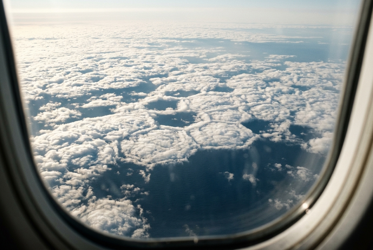
Cruising at 35,000 feet above the frigid expanses of the Labrador Sea in midwinter, the aircraft cabin is quiet, insulated from the violent thermodynamics unfolding five miles below. Press your forehead against the cold oval double-pane window, and the North Atlantic reveals one of the most mesmerizing visual spectacles on Earth: an immaculate, self-organizing geometric tapestry stretching from horizon to horizon.
Below, the ocean is not a featureless expanse of dark water, but a living lattice of cloud. In some sectors, the view resembles an endless sheet of bubble wrap or a sunlit field of white cobblestones—tightly packed, puffy cloud cushions separated by razor-thin ribbons of indigo sea. Several hundred miles to the south, the pattern abruptly inverts: the solid pillows give way to an intricate, lace-like honeycomb. Here, colossal hexagonal rings of towering cumulus frame cavernous, crystalline voids of clear air at their centers, resembling delicate doughnuts of water vapor arrayed with architectural precision across thousands of square kilometers.
Standing on a wind-whipped headland along the coast of Northern California or Brittany, you experience the terrestrial footprint of this same machinery. The air carries the sharp, saline tang of sea spray, and the breeze is remarkably steady, saturated with humidity. Looking westward toward the open ocean, the marine stratocumulus appears as a vast, unbroken grey ceiling—a low-slung, uniform blanket that keeps the coastal afternoon cool and muted. Yet satellite instruments orbiting hundreds of miles above reveal that this seemingly featureless deck is not uniform at all. It is a pulsating mosaic of mesoscale cellular convection, quietly executing an intricate dance of fluid mechanics governed by the exact same physical laws that make a heated saucepan of oil hum on a kitchen stove.
2. What’s Actually Happening — Plain English First
To understand why the maritime atmosphere organizes itself into these immense geometric networks, imagine a freshly poured cup of hot miso soup or a shallow pan of cooking oil warmed evenly over a low burner. If you look closely at the surface of the soup before stirring, you will notice miniature polygonal cells churning: tiny plumes of hot liquid rise in the center of each cell, spread outward across the surface, shed their heat to the surrounding room, and sink back down along the darker margins.
The atmosphere over the world’s oceans behaves in precisely the same manner, albeit on a gargantuan scale. The fluid medium is moist air, the "pan" is the planetary boundary layer—a relatively shallow sandwich of air typically one to two kilometers thick, bounded by the sea surface below and an invisible, lid-like temperature inversion above.
Think of the lower atmosphere as a massive thermal engine caught between two competing forces: buoyancy and resistance.
When a parcel of air is warmed by the relatively balmy sea surface beneath it, or cooled by radiating its heat out into the black void of space from its cloud tops, it develops a buoyancy mismatch with its neighbors. Warm, moist air wants to rise because it is less dense; cold, dry air wants to sink because it is heavier.
However, the air cannot move without friction. Viscosity (or more accurately, turbulent friction) and thermal diffusion constantly try to smear out these temperature differences and slow the motion down. Only when the thermal push becomes powerful enough to overcome the fluid's internal drag does the air break into organized circulatory loops.
Why do these loops take the form of distinct open and closed cells? The answer lies in where the engine is being driven:
- Closed Cells (Pillowy Centers, Clear Edges): Imagine a system driven primarily from the roof. Over the cool subtropical eastern oceans (such as off Peru, California, or Namibia), the cloud deck emits intense infrared radiation straight into outer space. This severe cloud-top cooling creates pockets of chilly, dense air at the upper boundary. These cold parcels sink along narrow perimeters, forcing a broad, gentle, moisture-laden updraft in the cell's center that condenses into a thick cloud dome.
- Open Cells (Clear Centers, Cloudy Walls): Now imagine a system driven forcefully from the floor. During a cold-air outbreak, when frigid Arctic air sweeps over the comparatively warm waters of the Gulf Stream or the Norwegian Sea, violent fluxes of heat and moisture boil upward from the ocean. This creates intense, concentrated updrafts that form towering cumulus clouds along the cell edges, while dry air from above sinks gently through the spacious, clear centers.
These convective structures are documented extensively by agencies such as the World Meteorological Organization and monitored continuously by NOAA Satellites to track boundary-layer dynamics across the globe.
3. The Science (For Those Who Want to Go Deeper)
To formalize the physics governing this atmospheric self-organization, we turn to classical hydrodynamic stability theory, first pioneered by Henri Bénard in 1900 and mathematically formalized by Lord Rayleigh in 1916. The fundamental question Rayleigh sought to answer was straightforward: Under what precise physical conditions will a resting layer of fluid, heated from below or cooled from above, become unstable and spontaneously initiate convective overturning?
The Classical Rayleigh-Bénard Problem and the Rayleigh Number
Rayleigh’s linear stability analysis of the Navier-Stokes equations under the Boussinesq approximation demonstrates that the onset of convection is governed by a single dimensionless parameter: the Rayleigh number ($Ra$).
The Rayleigh number represents the exact ratio between the buoyant forces destabilizing the fluid layer and the dissipative forces (viscous drag and thermal diffusion) working to restore equilibrium:
$$\Large Ra = \frac{g \beta \Delta T d^3}{\nu \kappa}$$
Where: * $g$ is the acceleration due to gravity ($9.81\text{ m s}^{-2}$). * $\beta$ is the thermal expansion coefficient of the fluid (for an ideal gas, $\beta = 1/T_0$, where $T_0$ is the mean absolute temperature in Kelvin). * $\Delta T$ is the vertical temperature difference across the fluid layer ($T_{\text{bottom}} - T_{\text{top}}$ in Kelvin). * $d$ is the geometric depth of the fluid layer (in meters). * $\nu$ is the kinematic molecular viscosity of the fluid ($\text{m}^2\text{ s}^{-1}$). * $\kappa$ is the thermal diffusivity of the fluid ($\text{m}^2\text{ s}^{-1}$).
In a classical laboratory setting bounded by two rigid, conducting horizontal plates, linear stability analysis proves that infinitesimal perturbations will decay exponentially if $Ra$ is small.
Only when the Rayleigh number exceeds a mathematically precise critical threshold:
$$\Large Ra_c \approx 1708$$
does the quiescent state lose stability, causing the fluid to spontaneously organize into stationary, counter-rotating convection rolls or hexagonal Bénard cells. For boundaries that are fluid and stress-free, this threshold drops to $Ra_c = \frac{27\pi^4}{4} \approx 657.5$.
For any fluid layer of depth $d$, convection cannot occur if $Ra < Ra_c$. When $Ra > Ra_c$, the kinetic energy generated by buoyancy per unit time exceeds the combined rate of viscous dissipation and thermal diffusion, initiating spontaneous fluid circulation.
Adapting Rayleigh-Bénard to the Atmospheric Boundary Layer
In the Earth's atmosphere, convection does not operate via molecular viscosity ($\nu \sim 1.5 \times 10^{-5}\text{ m}^2\text{ s}^{-1}$) or molecular thermal diffusivity ($\kappa \sim 2.1 \times 10^{-5}\text{ m}^2\text{ s}^{-1}$). If one were to insert molecular values into the atmospheric equation with a boundary layer depth of $d = 1000\text{ m}$, the calculated Rayleigh number would exceed $10^{16}$, implying uncontrollable turbulence.
Instead, the atmospheric boundary layer is governed by turbulent eddy viscosity ($K_m$) and turbulent eddy thermal diffusivity ($K_h$). Furthermore, atmospheric buoyancy is governed not merely by sensible temperature, but by the vertical gradient of virtual potential temperature ($\theta_v$), which accounts for both compressibility and the buoyant contribution of water vapor:
$$\Large Ra_{\text{turb}} = \frac{g}{\theta_{v0}} \frac{\Delta \theta_v \, z_i^3}{K_m K_h}$$
Where $z_i$ is the depth of the convective boundary layer (the height of the capping inversion), and $\theta_{v0}$ is the reference virtual potential temperature.
Worked Atmospheric Example: Marine Boundary Layer Convection
Let us calculate the turbulent Rayleigh number for a typical marine stratocumulus boundary layer over the Eastern Pacific:
- Boundary layer depth: $z_i = 1,200\text{ m}$
- Virtual potential temperature destabilization across layer: $\Delta \theta_v = 3.5\text{ K}$
- Mean boundary layer temperature: $\theta_{v0} = 288\text{ K}$
- Turbulent eddy momentum diffusivity: $K_m = 25\text{ m}^2\text{ s}^{-1}$
- Turbulent eddy thermal diffusivity: $K_h = 25\text{ m}^2\text{ s}^{-1}$
- Gravitational acceleration: $g = 9.81\text{ m s}^{-2}$
Step 1: Calculate the buoyant acceleration parameter: $$\frac{g}{\theta_{v0}} \Delta \theta_v = \frac{9.81}{288} \times 3.5 = 0.03406 \times 3.5 \approx 0.1192\text{ m s}^{-2}$$
Step 2: Calculate the volumetric scale factor ($z_i^3$): $$z_i^3 = (1,200\text{ m})^3 = 1.728 \times 10^9\text{ m}^3$$
Step 3: Calculate the turbulent dissipative product ($K_m K_h$): $$K_m K_h = 25\text{ m}^2\text{ s}^{-1} \times 25\text{ m}^2\text{ s}^{-1} = 625\text{ m}^4\text{ s}^{-2}$$
Step 4: Compute the turbulent Rayleigh number: $$Ra_{\text{turb}} = \frac{0.1192 \times (1.728 \times 10^9)}{625} = \frac{2.060 \times 10^8}{625} \approx 3.30 \times 10^5$$
Physical Interpretation: Because $Ra_{\text{turb}} \approx 3.3 \times 10^5 \gg Ra_c \approx 1708$, the marine boundary layer resides in a state of vigorous, fully developed turbulent cellular convection.
The Mesoscale Aspect Ratio Paradox
One of the greatest historical puzzles in meteorology is the discrepancy in aspect ratio (the ratio of horizontal cell diameter $L$ to vertical depth $d$, $\alpha = L/d$).
- Laboratory Rayleigh-Bénard Convection: Linear stability theory dictates that the fastest-growing convective wavenumber corresponds to a horizontal wavelength close to $L \approx 2\sqrt{2} d \approx 2.83 d$. Thus, laboratory aspect ratios are strictly isotropic, hovering between 1:1 and 3:1.
- Atmospheric Mesoscale Cellular Convection (MCC): High-resolution imagery from meteorological centers such as the Met Office and ECMWF reveals atmospheric cells with diameters ranging from 10 km to 40 km embedded within boundary layers that are only 1 km to 2 km deep. This corresponds to staggering aspect ratios between 10:1 and 30:1 (and occasionally up to 50:1).
Why does the atmosphere stretch its convective cells horizontally by an order of magnitude? Three dominant physical mechanisms account for this anomalous broadening:
1. Anisotropic Turbulent Eddy Diffusivity ($K_x, K_y \gg K_z$)
In the atmosphere, vertical motions are strictly constrained by the capping temperature inversion and the rigid sea surface. Horizontal turbulent motions, however, face no such spatial bounds. Consequently, horizontal eddy diffusivity ($K_h$) exceeds vertical eddy diffusivity ($K_z$) by orders of magnitude ($K_h / K_z \sim 10^2 - 10^3$).
Solving the modified perturbation equations with anisotropic diffusion coefficients reveals that the horizontal wavelength scales as:
$$L \sim d \sqrt{\frac{K_h}{K_z}}$$
This anisotropy stretches the circulation cells into wide, flattened pancakes.
2. Non-Local Cloud-Top Radiative Cooling and Inversion Entrainment
In closed-cell regimes, the primary driver of turbulence is not surface heating, but intense longwave radiative cooling at the cloud top. The cloud deck emits thermal infrared radiation to space at rates of $-50\text{ to }-80\text{ W m}^{-2}$ over a depth of just a few tens of meters.
This localized cooling produces narrow, negatively buoyant descending plumes that plunge downward through the cloud layer. As they sink, they entrain warm, dry air from across the capping inversion base, driving mesoscale baroclinic circulations that expand horizontally over tens of kilometers before ascending gently in the cell interior.
3. Precipitation Evaporation and Cold-Pool Dynamics in Open Cells
In open-cell regimes, cumulus clouds growing along the cell perimeters frequently produce drizzle. As this precipitation falls into the unsaturated sub-cloud layer, it evaporates, absorbing latent heat and creating cold, dense pools of downdraft air at the surface.
These divergent cold pools spread laterally across the sea surface like miniature gust fronts. When colliding with neighboring cold pools, they forcefully trigger new updrafts along their intersection lines, sustaining broad, cloud-free downdraft voids in the center while maintaining towering convective walls around perimeters 20 to 40 kilometers across.
| Convective Characteristic | Closed Mesoscale Cells | Open Mesoscale Cells |
|---|---|---|
| Typical Geographic Location | Eastern subtropical ocean basins (California, Peru, Canary currents) | Sub-polar maritime zones during Cold-Air Outbreaks (Labrador Sea, Sea of Japan) |
| Primary Thermodynamic Engine | Cloud-top longwave infrared cooling to space | Surface sensible and latent heat fluxes from warm ocean |
| Kinematic Structure | Broad, weak central updraft; narrow, intense peripheral downdrafts | Broad, gentle central downdraft; narrow, intense peripheral updrafts |
| Cloud Morphology | Stratocumulus decks filling 80–100% of cell area | Cumulus / Congestus rings filling 10–30% of cell area |
| Typical Aspect Ratio ($L/d$) | $15:1 \text{ to } 35:1$ ($L \sim 20\text{--}40\text{ km}$, $d \sim 1\text{--}1.5\text{ km}$) | $20:1 \text{ to } 40:1$ ($L \sim 30\text{--}50\text{ km}$, $d \sim 1.5\text{--}2.5\text{ km}$) |
| Precipitation Regime | Intermittent, light boundary-layer drizzle | Cellular rain showers, graupel, and localized squalls |
The mathematical formulation and classical proofs for these convective stability boundaries can be explored through the foundational literature archived on Wikipedia's Rayleigh-Bénard Convection Analysis and specialized atmospheric dynamics research hosted by NOAA Earth System Research Laboratories.
4. Practical Outdoor Guidance
While mesoscale cellular convection is most vividly resolved in satellite imagery, its presence and transitions exert profound, measurable influences on local weather, aviation conditions, and maritime operations.
What to Look for in the Sky
- From a Coastal Bluff or Ship at Sea: * Closed-Cell Stratocumulus: Look for a continuous, undulating grey-white deck with a defined, flat base typically between 1,500 and 3,000 feet above sea level. The sky feels uniformly overcast, yet the sun's disc may occasionally appear as a pale, diffuse silver coin through the thinner cell peripheries. * Open-Cell Transitions: If the uniform grey stratocumulus begins to fracture into distinct clusters with dark, towering cloud walls and sudden shafts of bright sunlight illuminating patches of open water, the boundary layer is transitioning to open cellular convection. You will observe dark rain or drizzle shafts trailing beneath the cell perimeters.
- From an Airline Window Seat: * When flying over maritime routes (e.g., London to New York or San Francisco to Honolulu), look straight down at the cloud deck. If the clouds resemble a tightly packed pavement of white stones with dark veins, you are above a closed-cell field. If the clouds form hollow, ring-like volcanic craters of white vapor around vast circular windows of blue ocean, you are viewing open-cell convection.
Instrument Readings to Watch
- Barometer (Atmospheric Pressure): Closed-cell decks are almost exclusively associated with high-pressure ridges and subtropical anticyclones (barometer reading typically steady between $1018\text{ hPa}$ and $1028\text{ hPa}$). Open-cell transitions accompany sharp drops in pressure ($1000\text{ hPa}$ to $1012\text{ hPa}$) following the passage of an ocean cold front.
- Thermometer and Dew Point Depression: In closed-cell regimes, the air temperature is cool and the dew point depression is negligible ($T - T_d < 1.5^\circ\text{C}$), reflecting high relative humidity near the surface. In open-cell regimes, the passage of a cell wall brings sudden drops in temperature of $2^\circ\text{C}\text{ to }4^\circ\text{C}$ due to evaporatively cooled downdrafts, accompanied by gusty, veering winds.
- Wind Direction and Gustiness: Under closed cells, surface winds are laminar and steady. Beneath open cells, surface winds become highly turbulent, pulsing with 15–25 knot gusts as the downdraft cold pools spread outward across the water.
Field Rules for Sailors, Aviators, and Hikers
- The Sailor’s Drizzle Rule: When sailing beneath an unbroken marine stratocumulus deck (closed cell), the onset of persistent, fine drizzle indicates that cloud-top radiative cooling has destabilized the inversion. Expect the cloud deck to thin or break up into cellular patches within the next 4 to 8 hours as precipitation cleanses the boundary layer of cloud droplets.
- The Aviator’s Turbulence Rule: Closed-cell decks provide smooth flight conditions above and below the cloud layer, with modest roll-vorticity turbulence confined entirely within the cloud stratum itself. Conversely, open-cell regimes feature vigorous, punchy vertical updrafts ($> 5\text{--}8\text{ m s}^{-1}$) within the cloudy perimeter walls, accompanied by moderate-to-severe boundary-layer icing hazards.
- The Coastal Hiker's Fog Clock: Along the Pacific coast or western European littoral, closed-cell decks push inland overnight as marine layer fog. When morning solar radiation warms the land, sensible heating drives the cell aspect ratio to expand, causing the cell centers to dissipate and the coastal fog to "burn off" from inland valleys toward the shoreline by midday.
5. Today’s Meteorological Rule of Thumb
When the ocean sky forms a solid quilt of white pillows, it is freezing from the top down; when it forms empty rings of towering cloud, it is boiling from the bottom up.
Whenever you see a fractured honeycomb of clouds out at sea or from the window of an airliner, remember that you are looking at nature's most elegant thermodynamic compromise: an entire ocean of air organizing itself into geometric corridors to transport heat from the planet’s surface into the cold infinity of space.