Quantum Volume: Quantifying Full-Stack Computational Capability and Circuit Depth in NISQ Processors
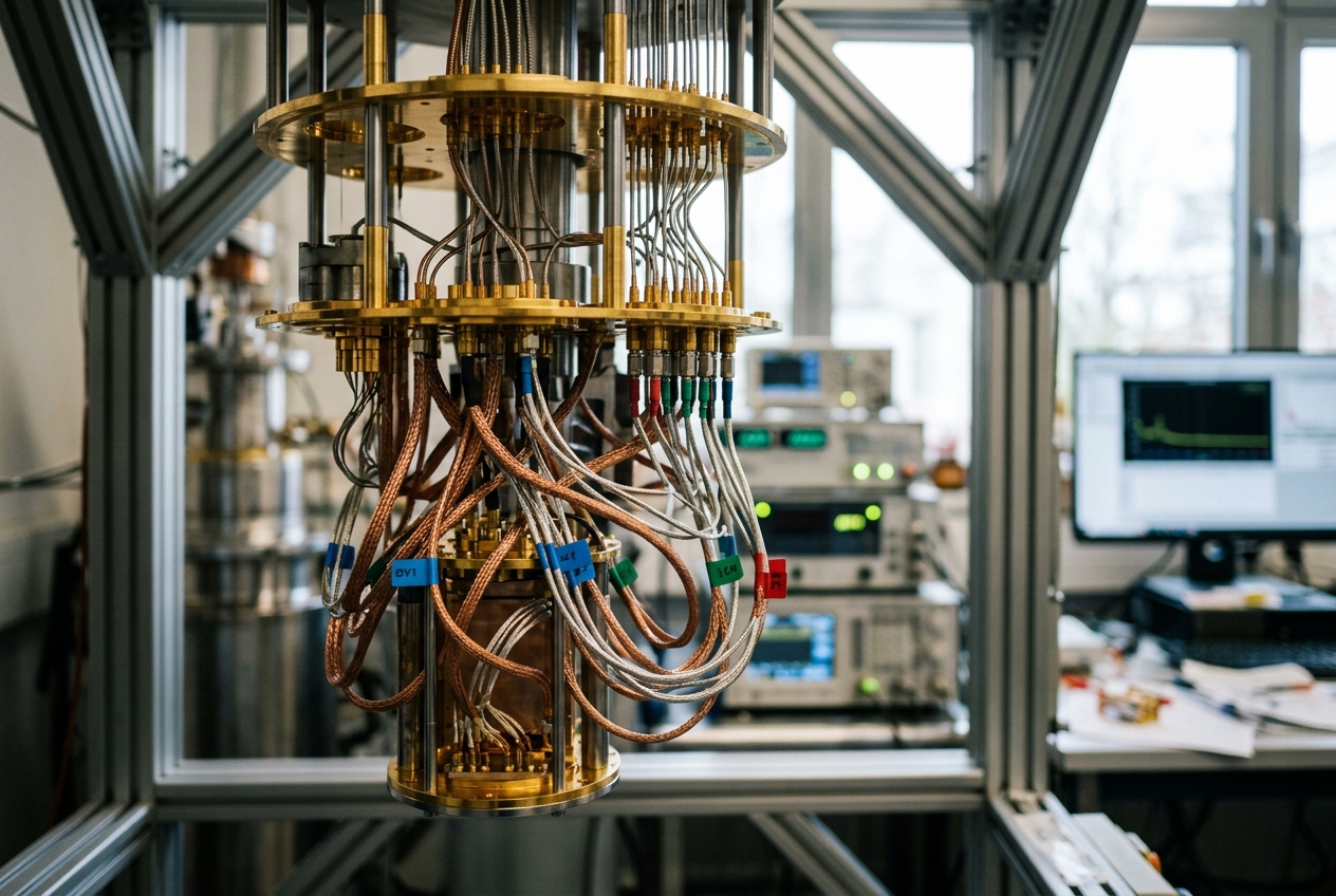
The stakes of this distinction could hardly be higher. The cryptographic foundations protecting the global financial architecture, confidential diplomatic communications, and personal digital identities rest upon mathematical problems—such as the factorization of large semiprimes—that would take conventional supercomputers millennia to unravel. A fully realised, fault-tolerant quantum computer could crack these algorithms in a matter of hours. Beyond cryptography, the same computational paradigm promises to unlock room-temperature superconductors, design bespoke catalysts for carbon capture, and simulate molecular dynamics for life-saving pharmaceuticals. But determining whether a quantum machine is genuinely approaching these transformative thresholds requires abandoning crude qubit headcounts in favour of a holistic, mathematically rigorous standard: Quantum Volume (QV).
1. The Idea in Plain English: Beyond the Spec Sheet
To understand why simply counting qubits is an illusion, consider an orchestral analogy. A musical ensemble cannot be judged solely by the number of musicians seated on stage. If half the violinists play out of tune, the brass section cannot hear the conductor’s tempo, and the percussionists are completely separated from the woodwinds by soundproof glass, adding five hundred more players will not produce a Beethoven symphony—it will merely generate an unbearable wall of acoustic noise. A compact, tightly coordinated chamber quartet playing in flawless harmony will achieve musical coherence that an undisciplined orchestra can never match.
In quantum mechanics, a quantum bit, or qubit, is not an immutable switch like a classical transistor that sits comfortably at a zero or a one. Instead, it is a delicate physical system—such as the energy levels of an artificial superconducting atom or the internal spin state of a trapped ion—existing in a continuum of simultaneous possibilities. When isolated from the world, a qubit can undergo delicate wave-like interference. However, four fundamental physical limitations constantly threaten to destroy this fragile computational state:
+-------------------------------------------------------------------------+
|                  THE FOUR VICES OF QUANTUM COMPUTATION                  |
+-------------------------------------------------------------------------+
| 1. Decoherence: The ambient thermal and electromagnetic leakage that    |
|    erases quantum information over time.                                |
| 2. Gate Errors: Tiny calibration inaccuracies when steering qubits with |
|    microwave or laser pulses.                                           |
| 3. Crosstalk: Unintended electromagnetic bleed where operating on one   |
|    qubit inadvertently perturbs its neighbours.                         |
| 4. Sparse Connectivity: Physical layout bottlenecks that prevent        |
|    arbitrary pairs of qubits from directly interacting.                 |
+-------------------------------------------------------------------------+
When quantum algorithms execute, they do not just spread across a line of physical qubits (which we call the system's width); they must also execute a sequence of successive operations over time (which we call the circuit's depth). If a machine possesses high width but abysmal depth, its computational capacity collapses before any meaningful calculation finishes.
Quantum Volume was formulated by researchers at IBM Quantum to capture this multifaceted reality. Rather than asking how many qubits exist on a chip, Quantum Volume asks a far more demanding question: What is the largest square box of quantum computation—equal parts width and depth—that this machine can execute successfully before noise annihilates the answer?
2. How It Actually Works: The Mechanics of Quantum Volume
To measure Quantum Volume, quantum engineers do not run cherry-picked algorithms tailored to a specific hardware layout. Instead, they subject the system to an unforgiving, randomised stress test designed to probe every single weakness simultaneously.
The Square Circuit Protocol
The protocol begins by choosing an arbitrary subset of $m$ active qubits from the total physical processor. The system is then tasked with executing an algorithm whose computational depth $d$ is deliberately set equal to its width: $d = m$. This creates an $m \times m$ "square circuit."
A single step of this circuit does not consist of simple, trivial pulses. Instead, the $m$ qubits are randomly paired off into disjoint couples. Each pair is subjected to an operation drawn uniformly at random from the special unitary group $\mathrm{SU}(4)$ via the Haar measure. In plain terms, an $\mathrm{SU}(4)$ unitary is the most general, maximally entangling two-qubit operation physically permissible under the laws of quantum mechanics. It scrambles the quantum information thoroughly across the two qubits.
At each subsequent depth step, the qubits are shuffled into a completely different, randomly chosen set of pairs, and another set of Haar-random $\mathrm{SU}(4)$ operations is applied. Because the pairings are chosen at random, two qubits that were across the chip in step one may be required to interact directly in step two. If the physical chip does not have direct physical wiring between those two qubits, the compiler must insert multiple intermediate swap operations—compounding the error rate and testing the machine's physical connectivity to its absolute limit.
Heavy Output Generation: Finding the Needle in the Quantum Haystack
Once the $m$ layers of random unitary operations have run, all $m$ qubits are measured simultaneously in the computational basis. The output is an $m$-bit binary string, such as $01101\dots1$.
Because the quantum circuit is composed of maximally scrambling, random operations, the ideal, noise-free output probabilities follow what physicists term a Porter-Thomas distribution. In such a distribution, the probabilities of obtaining different bitstrings are not uniformly flat; rather, a small subset of bitstrings has an exceptionally high probability of being observed, while the majority have an exceptionally low probability.
To evaluate whether the quantum computer executed the circuit faithfully, a classical computer simulates the exact same circuit in software and calculates the ideal probability distribution across all $2^m$ possible bitstrings. The classical simulator then computes the median probability $p_{\text{median}}$ of this ideal distribution.
Any bitstring whose ideal probability of occurrence is strictly greater than the median is designated a heavy output:
$$\mathcal{H} = \left{ x \in {0,1}^m : P_{\text{ideal}}(x) > p_{\text{median}} \right}$$
If the quantum computer were completely broken, acting as nothing more than a random noise generator, every bitstring would have an equal $1/2^m$ chance of appearing, and the probability of measuring a heavy output would be exactly $1/2$. Conversely, if the quantum hardware were mathematically flawless, integrating over the Porter-Thomas distribution reveals that the expected probability of measuring a heavy output converges to an elegant analytical constant:
$$h_{\text{ideal}} = \int_{\ln 2}^{\infty} p\, e^{-p} \, dp = \frac{1 + \ln 2}{2} \approx 0.8466$$
Probability Density
    ^
    |  *
    |  * *   Porter-Thomas Distribution
    |  *   *
    |  *     *  Ideal Heavy Output Area = ~84.66%
    |--*-------*-------------------------------------> Probability
       0    Median (ln 2)
       [-- Light --][----------- Heavy Output --------]
The 2/3 Success Threshold and Certification
A real-world quantum computer is neither completely noise-free nor purely random; it operates somewhere in between. To certify that a quantum processor has successfully mastered depth $m$, the experimental heavy output probability $h_m$ must not merely exceed $0.50$—it must surpass a strict mathematical threshold of two-thirds ($2/3 \approx 0.6667$).
Furthermore, because quantum mechanics is fundamentally probabilistic, this result cannot be an experimental fluke. The protocol requires running thousands of distinct random circuit instances, collecting tens of thousands of measurement shots, and establishing that the heavy output probability exceeds two-thirds with a $97.7\%$ statistical confidence level (corresponding to two standard deviations, or $2\sigma$, above the threshold).
The formal definition of Quantum Volume is given by the largest square circuit width $m$ that satisfies this strict condition:
$$\text{QV} = 2^m \quad \text{where} \quad m = \max \left{ k : h_k - 2\sigma_k > \frac{2}{3} \right}$$
When an experimental laboratory announces that they have achieved a Quantum Volume of $2^{16} = 65,536$ or $2^{20} = 1,048,576$, they are declaring that their hardware can reliably execute fully entangling, all-to-all randomised algorithms across $16$ or $20$ qubits through $16$ or $20$ consecutive layers of depth without succumbing to noise.
3. The Benchmarking Arena: How Quantum Volume Compares
Quantum Volume does not exist in an academic vacuum. It is part of a broader family of diagnostic metrics, each tailored to answer different questions about a quantum machine's health. Understanding its distinct role requires contrasting it with its prominent peers: Randomized Benchmarking and Cross-Entropy Benchmarking.
+-------------------------------------------------------------------------------------------------+
|                               COMPARATIVE BENCHMARKING TAXONOMY                                 |
+-----------------------------------+-----------------------------+-------------------------------+
| Metric                            | Target Domain               | Primary Blindspot             |
+-----------------------------------+-----------------------------+-------------------------------+
| Randomized Benchmarking (RB)      | Isolated 1- and 2-qubit     | Misses crosstalk, routing,    |
|                                   | gate fidelities             | and multi-qubit entanglement  |
+-----------------------------------+-----------------------------+-------------------------------+
| Cross-Entropy Benchmarking (XEB)  | Full-processor quantum      | Tied to native topology;      |
|                                   | supremacy sampling          | non-standardised depths       |
+-----------------------------------+-----------------------------+-------------------------------+
| Quantum Volume (QV)               | Holistic algorithmic        | Classical simulation wall     |
|                                   | power on square circuits    | beyond ~50 qubits             |
+-----------------------------------+-----------------------------+-------------------------------+
Randomized Benchmarking: The Component Check
Randomized Benchmarking (RB) is the micro-diagnostic of the quantum world. It isolates one or two qubits at a time and applies long sequences of randomly chosen Clifford gates, followed by an inversion gate that should return the qubits to their initial state. By measuring how fidelity decays as the sequence lengthens, physicists can extract average gate error rates (for instance, demonstrating a two-qubit gate fidelity of $99.8\%$).
However, RB suffers from a major structural limitation: it measures components in isolation. When all fifty or one hundred qubits on a chip operate simultaneously, microscopic electromagnetic fields bleed into adjacent transmission lines. This phenomenon, known as crosstalk, means that a two-qubit gate that exhibits $99.8\%$ fidelity in an isolated RB test might degrade to $96.0\%$ when the rest of the processor is firing. RB cannot capture these emergent, system-level failures; Quantum Volume captures them intrinsically.
Cross-Entropy Benchmarking: The Chaos Test
Cross-Entropy Benchmarking (XEB) gained global prominence through Google’s 2019 quantum supremacy demonstration on the Sycamore processor. Like Quantum Volume, XEB uses pseudo-random circuits to generate chaotic interference patterns and compares measured outputs against classically computed probability distributions.
The fundamental difference lies in structure and intent. XEB was conceived to demonstrate that a specific, physical chip topology could produce an output distribution that no classical supercomputer could sample within a reasonable timeframe. To achieve this, XEB circuits are mapped directly onto the native, nearest-neighbour grid of the physical hardware, avoiding the need for complex qubit routing.
Quantum Volume, by contrast, enforces arbitrary, all-to-all logical connectivity through random permutations. This deliberately forces the compiler to route qubits across the chip, making QV an uncompromising test of general-purpose algorithmic utility rather than a specialised hardware showcase.
4. The Architectural Crucible: Topologies and Compilers
The insistence on random permutations highlights one of the most critical factors in modern quantum architecture: the relationship between hardware topology and compiler optimization.
Sparse Lattices versus All-to-All Connectivity
In superconducting quantum circuits—the technology championed by IBM and Google—qubits are lithographically patterned onto a two-dimensional silicon chip. Physical considerations, particularly the density of control wiring and parasitic frequency collisions, strictly limit connectivity. IBM’s widely adopted heavy-hexagonal lattice, for instance, places qubits along the vertices and edges of hexagons, meaning most qubits can directly interact with only two or three physical neighbours.
       Superconducting Heavy-Hex (Sparse)            Trapped-Ion Architecture (All-to-All)
               Q --- Q --- Q                                      [ Ion 1 ]
              /             \                                    /    |    \
             Q               Q                            [ Ion 4 ] --+-- [ Ion 2 ]
              \             /                                    \    |    /
               Q --- Q --- Q                                      [ Ion 3 ]
        (Interactions require SWAP chains)             (Arbitrary laser-mediated coupling)
In sharp contrast, trapped-ion architectures—such as those engineered by Quantinuum—suspend individual charged ytterbium or barium atoms in an ultra-high vacuum using radiofrequency electric fields. By steering focused laser beams or physically shuttling the ions across an electromagnetic track, any arbitrary pair of qubits can be entangled directly, providing near-perfect all-to-all connectivity.
The Heavy Toll of SWAP Overhead
When a Quantum Volume test demands an $\mathrm{SU}(4)$ interaction between two qubits situated on opposite sides of a planar grid, the quantum compiler (such as Qiskit) must synthesize a bridge. It does this by inserting a sequence of SWAP gates—each composed of three consecutive controlled-NOT (CNOT) operations—to mechanically transport the quantum state across the chip and back.
$$P_{\text{success}} \approx \exp\left( - C \cdot m^2 \cdot \epsilon \right)$$
A modest error rate that seems tolerable in isolated tests rapidly drives the heavy output probability below the critical $2/3$ threshold as $m$ grows.
This mathematical reality explains why trapped-ion systems with all-to-all connectivity have consistently set world records in Quantum Volume (reaching certified volumes of $2^{20}$ and beyond), despite having fewer total physical qubits than massive superconducting arrays. The absence of routing overhead allows the physical depth to match the logical depth exactly.
5. Scaling Bottlenecks in the Pre-Fault-Tolerant Era
As quantum computing progresses through the Noisy Intermediate-Scale Quantum (NISQ) era toward early fault tolerance, Quantum Volume faces two formidable physical and computational boundaries:
- The Physical Error Floor: To advance from a Quantum Volume of $2^6$ (64) to $2^{20}$ (1,048,576), a processor's physical two-qubit error rates must plummet from approximately $1\%$ ($10^{-2}$) to well below $0.01\%$ ($10^{-4}$). Without active quantum error correction, residual environmental decoherence and drift inevitably cap the maximum achievable volume.
- The Classical Verification Wall: The second bottleneck is philosophical and computational. Calculating the heavy output set $\mathcal{H}$ requires an exact classical simulation of the $m \times m$ circuit. Because state-vector simulation of an arbitrary quantum system scales exponentially as $\mathcal{O}(2^m)$, verifying a Quantum Volume of $2^{50}$ would demand simulating a 50-qubit Haar-random circuit—requiring petabytes of RAM and days of supercomputer execution time. Beyond roughly 55 to 60 qubits, exact classical verification becomes mathematically and physically intractable.
Consequently, Quantum Volume serves as the ultimate diagnostic benchmark for the NISQ and early logical-qubit era, providing an empirical bridge until the industry fully transitions to large-scale error-corrected architectures evaluated by logical benchmarks.
6. Real-World Applications Today (2024–2026)
The pursuit of high Quantum Volume is not merely a metrological exercise. Across global research laboratories and industrial consortia, systems certified with high Quantum Volume are being deployed to tackle real-world computational bottlenecks where noise resilience is paramount.
+---------------------------------------------------------------------------------------------------+
|                           FRONTIER INDUSTRIAL DEPLOYMENTS (2024–2026)                             |
+--------------------------+-----------------------+------------------------------------------------+
| Organization             | Domain                | Quantum Advantage Mechanism                    |
+--------------------------+-----------------------+------------------------------------------------+
| BMW Group & Quantinuum   | Materials Science &   | Simulating platinum-catalyst chemical kinetics |
|                          | Battery Chemistry     | with deeply entangled state preparation        |
+--------------------------+-----------------------+------------------------------------------------+
| JPMorgan Chase & IBM     | Quantitative Finance  | Executing multi-asset portfolio optimization   |
|                          | & Risk Analysis       | using high-depth QAOA variational circuits     |
+--------------------------+-----------------------+------------------------------------------------+
| Cleveland Clinic & IBM   | Biomedical Genomics   | Computing quantum kernel spaces for pathogen   |
|                          | & Structural Biology  | structural variant classification              |
+--------------------------+-----------------------+------------------------------------------------+
| QuEra & Harvard/MIT      | Quantum Simulation    | Coherent spatial atom shuttling for non-local  |
|                          | & Neutral Atoms       | combinatorial graph optimisation               |
+--------------------------+-----------------------+------------------------------------------------+
1. High-Fidelity Quantum Chemistry and Catalysis
In collaboration with Quantinuum, researchers at the BMW Group and Airbus have utilized ultra-high Quantum Volume trapped-ion processors (such as the H1 and H2 series) to simulate the reaction pathways of oxygen reduction on platinum-based catalysts for fuel cells. Simulating these strongly correlated electron systems on classical computers requires severe approximations. The high Quantum Volume of the hardware enables deep unitary circuits that maintain entanglement long enough to capture exact electronic ground-state energies.
2. Algorithmic Portfolio Optimization and Risk Modelling
In the financial sector, teams at JPMorgan Chase working with IBM Quantum have implemented advanced variants of the Quantum Approximate Optimization Algorithm (QAOA). High-dimensional portfolio optimization problems require dense inter-asset correlations, translating to circuits with extensive multi-qubit entanglement. Running these algorithms on processors with high Quantum Volume ensures that the resulting optimization landscapes are not smoothed out by gate errors, yielding viable non-classical solutions.
3. Structural Biology and Pathogen Genomics
At the Cleveland Clinic’s Center for Computational Life Sciences, researchers are leveraging high-QV superconducting quantum processors to develop quantum machine learning models for genomic analysis. By encoding complex molecular interactions into high-dimensional quantum kernel spaces, researchers are mapping the evolutionary fitness landscapes of viral mutations. High circuit fidelity ensures that subtle topological features in the genomic data are preserved during quantum state preparation.
4. Neutral Atom Quantum Computing
Institutions such as QuEra Computing, in partnership with researchers from Harvard University and MIT OpenCourseWare, are advancing neutral-atom architectures that rely on optical tweezers to shuttle rubidium atoms in real time. Benchmarking these systems against the principles of Quantum Volume demonstrates how dynamic physical rearrangement can bypass the connectivity limits of static planar lattices, setting new records in effective computational depth.
7. What This Means for You
For the non-specialist observing the evolution of quantum technology, the lessons of Quantum Volume offer a vital lens through which to interpret the future:
- Demystifying Cryptographic Timelines: Whenever a headline warns that "Quantum Computers Will Break the Internet Next Year," look past the qubit count. Breaking 2048-bit RSA encryption does not just require 4,000 raw qubits; it requires a machine capable of executing algorithms with billions of coherent, fault-tolerant gate operations. Understanding Quantum Volume shows that we remain in the NISQ validation regime, giving society crucial time to transition to post-quantum cryptography.
- Accelerating the Green Energy Transition: The design of high-temperature electrical grids, solid-state battery electrolytes, and industrial nitrogen fixation (which currently consumes several percent of all global natural gas via the classical Haber-Bosch process) depends directly on the depth of quantum chemical simulations. Incremental increases in Quantum Volume directly translate into more accurate chemical simulations, accelerating the discovery of sustainable materials.
- An Antidote to Tech Hype: In an era rife with exaggerated claims, Quantum Volume provides a clear, quantitative yardstick. It reminds us that meaningful computational progress is driven not by superficial scaling, but by systemic precision, interconnectivity, and error suppression.