Quantum Process Tomography: Reconstructing Dynamical Superoperators and Process Matrices in Quantum Circuits
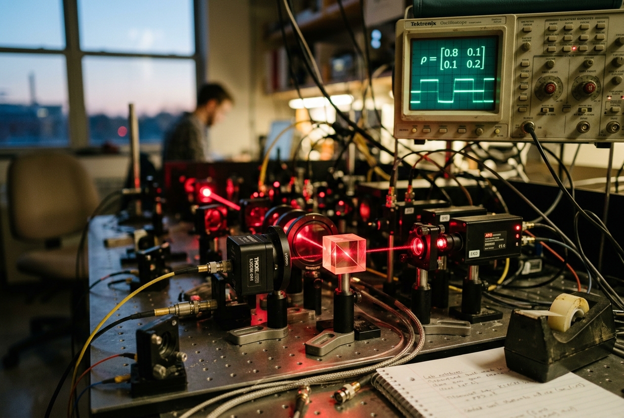
To diagnose, calibrate, and error-correct physical quantum hardware—from superconducting transmons to trapped ions—physicists require a rigorous mathematical and experimental framework to reconstruct the full transfer matrix of any unknown quantum operation. This diagnostic technique is Quantum Process Tomography (QPT).
While Quantum State Tomography (QST) reconstructs the static density matrix $\rho$ of a prepared system, QPT fully characterizes the underlying dynamical map $\mathcal{E}$ itself. By probing the quantum channel with an informationally complete ensemble of input states and reconstructing the corresponding output states, QPT extracts the complete microscopic representation of gate errors, environmental damping, and coherent phase drifts.
1. From State Characterization to Channel Reconstruction
1.1 The Inadequacy of State Tomography for Dynamical Diagnosis
Quantum State Tomography operates on an ensemble of identically prepared quantum systems in an unknown density matrix $\rho \in \mathcal{H}d$, where $d = 2^n$ is the Hilbert space dimension for an $n$-qubit register. By measuring expectation values $\langle M_k \rangle = \mathrm{Tr}(M_k \rho)$ over a quorum of informationally complete measurement operators ${M_k}{k=1}^{d^2}$, the state $\rho$ is reconstructed.
However, observing a static output state $\rho_{\text{out}} = \mathcal{E}(\rho_{\text{in}})$ for a single input state reveals only how the channel acts on that specific state vector. If a quantum gate is subjected to systematic miscalibration—such as an over-rotation along an orthogonal axis—evaluating a single input like $|0\rangle$ might mask errors that manifest acutely on superpositions such as $|+\rangle = \frac{1}{\sqrt{2}}(|0\rangle + |1\rangle)$. Complete operational diagnostics require determining how $\mathcal{E}$ transforms every linear operator in the operator space $\mathcal{L}(\mathcal{H})$.
                    QUANTUM PROCESS TOMOGRAPHY WORKFLOW

   +-----------------------------------------------------------------+
   | 1. Prepare Informationally Complete Inputs {ρ_j} (j = 1...d²)    |
   +-----------------------------------------------------------------+
                                    |
                                    v
   +-----------------------------------------------------------------+
   | 2. Pass Each State Through the Unknown Quantum Channel E(ρ_j)   |
   +-----------------------------------------------------------------+
                                    |
                                    v
   +-----------------------------------------------------------------+
   | 3. Perform Full State Tomography (QST) on Each Output Channel   |
   |    Measure Quorum of Observables {M_k}                          |
   +-----------------------------------------------------------------+
                                    |
                                    v
   +-----------------------------------------------------------------+
   | 4. Invert System / Perform Constrained Optimization (MLE / SDP) |
   |    Enforce Complete Positivity & Trace Preservation (CPTP)      |
   +-----------------------------------------------------------------+
                                    |
                                    v
   +-----------------------------------------------------------------+
   | 5. Extract Process Matrix χ, Kraus Operators, and Gate Fidelity  |
   +-----------------------------------------------------------------+
1.2 Mathematical Formulation of Completely Positive Trace-Preserving (CPTP) Maps
Any physical, linear, memoryless quantum operation is mathematically defined as a linear superoperator mapping the space of density operators to itself:
$$\mathcal{E}: \mathcal{L}(\mathcal{H}_d) \longrightarrow \mathcal{L}(\mathcal{H}_d)$$
For $\mathcal{E}$ to represent a physically realizable quantum process, it must satisfy two fundamental constraints: 1. Trace Preservation (TP): Total probability is conserved: $$\mathrm{Tr}(\mathcal{E}(\rho)) = \mathrm{Tr}(\rho) = 1, \quad \forall \rho \in \mathcal{L}(\mathcal{H}d)$$ 2. Complete Positivity (CP): The map must preserve positivity not only on $\mathcal{H}_d$, but also when extended to an arbitrary composite system $\mathcal{H}_d \otimes \mathcal{H}_E$ of arbitrary dimension $d_E$: $$(\mathcal{E} \otimes \mathcal{I}{d_E})(\rho_{SE}) \succeq 0, \quad \forall \rho_{SE} \ge 0$$
Positivity alone (mapping positive operators to positive operators on $\mathcal{H}$) is insufficient; non-completely positive maps, such as the matrix transpose operation $T(\rho) = \rho^T$, generate unphysical negative probabilities when applied locally to an entangled state.
To reconstruct $\mathcal{E}$, we construct an Informationally Complete Basis of density matrices ${\rho_j}{j=1}^{d^2}$ spanning $\mathcal{L}(\mathcal{H}_d)$. Because $\mathcal{E}$ is a linear mapping, its action on an arbitrary input state $\rho = \sum{j=1}^{d^2} c_j \rho_j$ is uniquely determined by linearity:
$$\mathcal{E}(\rho) = \sum_{j=1}^{d^2} c_j \mathcal{E}(\rho_j)$$
Hence, running QST on the $d^2$ outputs ${\mathcal{E}(\rho_j)}$ yields sufficient data to fully characterize the dynamical channel.
2. Operator-Basis Expansion, the Process Matrix $\chi$, and Fundamental Isomorphisms
2.1 The Pauli Operator-Basis Expansion
Let ${E_m}{m=0}^{d^2-1}$ be a fixed, orthonormal basis for the space of operators $\mathcal{L}(\mathcal{H}_d)$ with respect to the Hilbert-Schmidt inner product $\langle A, B \rangle{\text{HS}} = \mathrm{Tr}(A^\dagger B)$, satisfying:
$$\mathrm{Tr}(E_m^\dagger E_n) = d \, \delta_{mn}$$
For an $n$-qubit register ($d=2^n$), the natural choice is the $n$-fold tensor product of Pauli operators ${I, X, Y, Z}^{\otimes n}$. Because ${E_m}$ forms an operator basis, any quantum operation acting on an arbitrary density matrix $\rho$ can be uniquely parameterized as:
$$\mathcal{E}(\rho) = \sum_{m=0}^{d^2-1} \sum_{n=0}^{d^2-1} \chi_{mn} E_m \rho E_n^\dagger$$
The complex matrix $\chi \in \mathbb{C}^{d^2 \times d^2}$ is known as the process matrix (or $\chi$-matrix). The $\chi$-matrix contains $d^4 = 16^n$ real parameters before applying physical constraints.
2.2 Algebraic Constraints on the Process Matrix
The physical mandates on $\mathcal{E}$ impose direct algebraic structures onto $\chi$:
-
Hermiticity: Since $\mathcal{E}(\rho^\dagger) = (\mathcal{E}(\rho))^\dagger$, the process matrix is strictly Hermitian: $$\chi = \chi^\dagger \implies \chi_{mn} = \chi_{nm}^*$$
-
Complete Positivity: According to the Choi-Jamiołkowski Isomorphism, $\mathcal{E}$ is completely positive if and only if $\chi$ is positive semidefinite: $$\chi \succeq 0 \iff \langle v | \chi | v \rangle \ge 0, \quad \forall |v\rangle \in \mathbb{C}^{d^2}$$
-
Trace Preservation: For all $\rho$, $\mathrm{Tr}(\mathcal{E}(\rho)) = \mathrm{Tr}(\rho)$. Expanding $\mathcal{E}(\rho)$ yields: $$\mathrm{Tr}\left(\sum_{m,n} \chi_{mn} E_m \rho E_n^\dagger\right) = \mathrm{Tr}\left(\rho \sum_{m,n} \chi_{mn} E_n^\dagger E_m\right) = \mathrm{Tr}(\rho)$$ Because this must hold for all arbitrary density matrices $\rho$, the operator completeness condition emerges: $$\sum_{m=0}^{d^2-1} \sum_{n=0}^{d^2-1} \chi_{mn} E_n^\dagger E_m = I_d$$
Taking the expectation value with respect to the operator basis yields $d^2$ linear equality constraints, reducing the number of independent real parameters of a general $n$-qubit CPTP channel to:
$$N_{\text{params}} = d^2(d^2 - 1) = 4^n(4^n - 1)$$
For a single qubit ($n=1$), $N_{\text{params}} = 4 \times 3 = 12$ independent parameters (down from 16). For a two-qubit gate ($n=2$), $N_{\text{params}} = 16 \times 15 = 240$ parameters.
+----------------------------------------------------------------------------------------------------+
|                               CANONICAL CHANNEL REPRESENTATIONS                                    |
+----------------------------------------------------------------------------------------------------+
| 1. Process Matrix (χ):         E(ρ) = ∑_{m,n} χ_{mn} E_m ρ E_n†                                    |
| 2. Kraus Representation:       E(ρ) = ∑_k A_k ρ A_k†,    where A_k = √λ_k ∑_m v_{k,m} E_m          |
| 3. Choi Matrix (Λ_E):          Λ_E = (E ⊗ I)(|Φ+⟩⟨Φ+|) = (1/d) ∑_{m,n} χ_{mn} (E_m ⊗ I)|Φ+⟩⟨Φ+|... |
| 4. Liouville / Superoperator:  |E(ρ)⟩⟩ = S |ρ⟩⟩,         S_{ij} = (1/d) Tr(E_i† E(E_j))            |
+----------------------------------------------------------------------------------------------------+
2.3 Direct Connection to Kraus Representation and Choi State
The process matrix $\chi$ connects directly to the Kraus Representation Theorem and the Choi-Jamiołkowski Isomorphism.
By the spectral theorem, since $\chi \succeq 0$, it admits an eigendecomposition:
$$\chi = \sum_{k=1}^{r} \lambda_k |v_k\rangle \langle v_k|, \quad \lambda_k \ge 0, \quad r \le d^2$$
where $|v_k\rangle = \sum_{m=0}^{d^2-1} v_{k,m} |m\rangle$ are the orthonormal eigenvectors of $\chi$, and $r = \mathrm{rank}(\chi)$ is the Kraus rank of the channel. Substituting this decomposition back into the operator expansion:
$$\mathcal{E}(\rho) = \sum_{m,n=0}^{d^2-1} \left( \sum_{k=1}^r \lambda_k v_{k,m} v_{k,n}^* \right) E_m \rho E_n^\dagger = \sum_{k=1}^r \left( \sqrt{\lambda_k} \sum_m v_{k,m} E_m \right) \rho \left( \sqrt{\lambda_k} \sum_n v_{k,n} E_n \right)^\dagger$$
Defining the set of Kraus operators ${A_k}_{k=1}^r$ as:
$$A_k = \sqrt{\lambda_k} \sum_{m=0}^{d^2-1} v_{k,m} E_m$$
we recover the canonical Kraus Representation:
$$\mathcal{E}(\rho) = \sum_{k=1}^r A_k \rho A_k^\dagger, \quad \text{with} \quad \sum_{k=1}^r A_k^\dagger A_k = I_d$$
Similarly, the Choi state $\Lambda_{\mathcal{E}} \in \mathcal{L}(\mathcal{H}A \otimes \mathcal{H}_B)$ is defined by applying the channel $\mathcal{E}$ to one half of a maximally entangled state $|\Phi^+\rangle = \frac{1}{\sqrt{d}}\sum{i=0}^{d-1} |i\rangle \otimes |i\rangle$:
$$\Lambda_{\mathcal{E}} = (\mathcal{E} \otimes \mathcal{I})(|\Phi^+\rangle \langle \Phi^+|) = \frac{1}{d} \sum_{i,j=0}^{d-1} \mathcal{E}(|i\rangle\langle j|) \otimes |i\rangle\langle j|$$
The Choi matrix $\Lambda_{\mathcal{E}}$ is related to $\chi$ by an explicit change of basis:
$$\Lambda_{\mathcal{E}} = \frac{1}{d} \sum_{m,n=0}^{d^2-1} \chi_{mn} (E_m \otimes I) |\Phi^+\rangle \langle \Phi^+| (E_n^\dagger \otimes I)$$
Complete positivity of $\mathcal{E}$ is equivalent to $\Lambda_{\mathcal{E}} \succeq 0$, and trace preservation corresponds to the partial trace condition $\mathrm{Tr}A(\Lambda{\mathcal{E}}) = \frac{1}{d} I_B$. For more details, consult the foundational literature in Nature Physics and course notes from MIT OpenCourseWare Quantum Information Science.
3. Explicit Analytic Derivation for Single-Qubit Process Tomography
To illustrate the algebraic machinery, consider a single-qubit channel ($d=2$). We select the standard normalized Pauli operator basis:
$$E_0 = I = \begin{pmatrix} 1 & 0 \ 0 & 1 \end{pmatrix}, \quad E_1 = X = \begin{pmatrix} 0 & 1 \ 1 & 0 \end{pmatrix}, \quad E_2 = Y = \begin{pmatrix} 0 & -i \ i & 0 \end{pmatrix}, \quad E_3 = Z = \begin{pmatrix} 1 & 0 \ 0 & -1 \end{pmatrix}$$
satisfying $\mathrm{Tr}(E_m E_n) = 2 \, \delta_{mn}$.
                             SINGLE-QUBIT TOMOGRAPHY QUORUM

             |0⟩ (Z+) ----------------------------> E(|0⟩⟨0|) ---> [X, Y, Z Measurements]
             |1⟩ (Z-) ----------------------------> E(|1⟩⟨1|) ---> [X, Y, Z Measurements]
    |+⟩ = (|0⟩+|1⟩)/√2 (X+) ---------------------> E(|+⟩⟨+|) ---> [X, Y, Z Measurements]
  |+i⟩ = (|0⟩+i|1⟩)/√2 (Y+) --------------------> E(|+i⟩⟨+i|) --> [X, Y, Z Measurements]
3.1 Input State Quorum and Output Decompositions
We prepare $d^2 = 4$ linearly independent pure input states spanning $\mathcal{L}(\mathcal{H}_2)$: 1. $\rho_1 = |0\rangle\langle 0| = \begin{pmatrix} 1 & 0 \ 0 & 0 \end{pmatrix} = \frac{1}{2}(I + Z)$ 2. $\rho_2 = |1\rangle\langle 1| = \begin{pmatrix} 0 & 0 \ 0 & 1 \end{pmatrix} = \frac{1}{2}(I - Z)$ 3. $\rho_3 = |+\rangle\langle +| = \frac{1}{2}\begin{pmatrix} 1 & 1 \ 1 & 1 \end{pmatrix} = \frac{1}{2}(I + X)$ 4. $\rho_4 = |+i\rangle\langle +i| = \frac{1}{2}\begin{pmatrix} 1 & -i \ i & 1 \end{pmatrix} = \frac{1}{2}(I + Y)$
Each state $\rho_j$ is injected into the channel $\mathcal{E}$, and full quantum state tomography is executed on the output $\rho_j' = \mathcal{E}(\rho_j)$. The output states are parameterized in the Pauli basis via Stokes parameters:
$$\rho_j' = \mathcal{E}(\rho_j) = \frac{1}{2} \sum_{k=0}^3 S_{jk} E_k, \quad \text{where } S_{jk} = \mathrm{Tr}(E_k \mathcal{E}(\rho_j))$$
3.2 Linear System Formulation
Using the process expansion $\mathcal{E}(\rho_j) = \sum_{m,n=0}^3 \chi_{mn} E_m \rho_j E_n^\dagger$, we expand each matrix product $E_m \rho_j E_n^\dagger$ in the Pauli basis:
$$E_m \rho_j E_n^\dagger = \sum_{k=0}^3 \Gamma_{jk}^{mn} E_k, \quad \text{where } \Gamma_{jk}^{mn} = \frac{1}{2} \mathrm{Tr}\left( E_k E_m \rho_j E_n^\dagger \right)$$
Equating the coefficients of $E_k$ across the experimental outputs gives:
$$\frac{1}{2} S_{jk} = \sum_{m,n=0}^3 \chi_{mn} \Gamma_{jk}^{mn}$$
Vectorizing the $4 \times 4$ process matrix $\chi$ into a 16-dimensional vector $\vec{\chi} \in \mathbb{C}^{16}$ and flattening the indices $(j, k)$ into a 16-dimensional measurement vector $\vec{S} \in \mathbb{R}^{16}$, we obtain the linear system:
$$\vec{S} = M \vec{\chi}$$
where $M \in \mathbb{C}^{16 \times 16}$ is the fixed transformation matrix computed purely from the algebra of Pauli matrices and input states. Inverting $M$ provides the direct linear inversion solution:
$$\vec{\chi}_{\text{raw}} = M^{-1} \vec{S}$$
4. The Sampling Noise Breakdown: Maximum Likelihood Estimation and Semidefinite Programming
4.1 Unphysical Solutions from Linear Inversion
In an idealized, noise-free experiment with infinite measurement shots, $\vec{\chi}_{\text{raw}} = M^{-1} \vec{S}$ yields an exact, positive semidefinite process matrix.
However, experimental measurements on quantum processors are subject to finite-shot statistical fluctuations (multinomial projection noise) and State Preparation and Measurement (SPAM) errors. As a result, the measured vector $\vec{S}{\text{exp}} = \vec{S}{\text{true}} + \vec{\epsilon}$ deviates from the valid quantum simplex.
Direct linear inversion of noisy experimental data frequently produces a $\chi_{\text{raw}}$ matrix with negative eigenvalues, violating complete positivity ($\chi \not\succeq 0$). An unphysical $\chi$ cannot be converted into Kraus operators and predicts negative probabilities for certain test states.
       EXPERIMENTAL DATA AND CONSTRAINED ESTIMATION MANIFOLD

              [ Unconstrained Inversion χ_raw ] (Contains negative eigenvalues)
                            |
                            | Projection / Likelihood Maximization
                            v
       +-------------------------------------------------------------+
       |   PHYSICAL MANIFOLD OF QUANTUM CHANNELS                     |
       |                                                             |
       |   Complete Positivity:  χ ⪰ 0 (Cone of PSD matrices)        |
       |   Trace Preservation:   ∑_{m,n} χ_{mn} E_n† E_m = I         |
       |                                                             |
       |          [ Optimal Physical Estimate χ_MLE / χ_SDP ]        |
       +-------------------------------------------------------------+
4.2 Maximum Likelihood Estimation (MLE) via Cholesky Parameterization
To enforce complete positivity by construction, Maximum Likelihood Estimation parameterizes the process matrix through its matrix square root. Any positive semidefinite matrix $\chi$ can be written in Cholesky-factored form:
$$\chi(T) = \frac{T^\dagger T}{\mathrm{Tr}(T^\dagger T)}$$
where $T$ is a lower triangular complex matrix:
$$T = \begin{pmatrix} t_1 & 0 & 0 & \dots & 0 \ t_2 + i t_3 & t_4 & 0 & \dots & 0 \ t_5 + i t_6 & t_7 + i t_8 & t_9 & \dots & 0 \ \vdots & \vdots & \vdots & \ddots & \vdots \end{pmatrix}$$
Under this parameterization, $\chi(T)$ is guaranteed to be Hermitian and positive semidefinite ($\chi \succeq 0$) for any choice of real parameters $\vec{t} \in \mathbb{R}^{d^4}$.
The trace-preservation constraint $\sum_{m,n} \chi_{mn}(T) E_n^\dagger E_m = I$ is enforced either as a Lagrange multiplier or as a constrained manifold optimization.
Given measurement outcomes where basis state $\rho_j$ yielded measurement operator $M_a$ with count $n_{ja}$ over $N_{\text{shots}}$ trials, the likelihood function is:
$$\mathcal{L}(T) = \prod_{j=1}^{d^2} \prod_{a=1}^{d^2} \left[ P(a | \rho_j, T) \right]^{n_{ja}}, \quad P(a | \rho_j, T) = \mathrm{Tr}\left( M_a \mathcal{E}_T(\rho_j) \right)$$
Minimizing the negative log-likelihood:
$$\min_{\vec{t}} f(\vec{t}) = -\sum_{j,a} n_{ja} \ln \left( \mathrm{Tr}\left( M_a \sum_{m,n} \chi_{mn}(T) E_m \rho_j E_n^\dagger \right) \right)$$
yields an optimal, physically valid estimate $\chi_{\text{MLE}}$.
4.3 Convex Formulation via Semidefinite Programming (SDP)
Alternatively, constrained linear least-squares can be cast as a Semidefinite Program (SDP), guaranteeing convergence to a global minimum without local trapping:
$$\begin{aligned} \min_{\chi} \quad & | M \vec{\chi} - \vec{S}{\text{exp}} |_2^2 \ \text{subject to} \quad & \chi \succeq 0, \ & \sum{m,n=0}^{d^2-1} \chi_{mn} \mathrm{Tr}(E_n^\dagger E_m E_k) = d \, \delta_{k0}, \quad \forall k \in {0, \dots, d^2-1} \end{aligned}$$
SDP methods scale efficiently for 1- and 2-qubit systems and are standard in modern quantum packages like Qiskit and Physical Review Letters publications.
5. The Exponential Bottleneck and Scalable Diagnostic Alternatives
5.1 The Curse of Dimensionality in Standard QPT
Despite its diagnostic completeness, standard QPT suffers from an exponential scaling bottleneck that renders it intractable for registers beyond 3 or 4 qubits:
| Qubit Count ($n$) | Hilbert Dim ($d=2^n$) | Input States ($4^n$) | Measurement Settings ($6^n$ Pauli) | Free Parameters ($4^n(4^n-1)$) |
|---|---|---|---|---|
| 1 | 2 | 4 | 6 | 12 |
| 2 | 4 | 16 | 36 | 240 |
| 3 | 8 | 64 | 216 | 3,840 |
| 4 | 16 | 256 | 1,296 | 61,440 |
| 5 | 32 | 1,024 | 7,776 | 983,040 |
| 10 | 1,024 | $1.05 \times 10^6$ | $6.05 \times 10^7$ | $\approx 1.10 \times 10^{12}$ |
For an $n$-qubit register, full QPT requires preparing $4^n$ states and measuring $3^n$ configurations per state, giving $12^n$ total circuit executions.
Furthermore, QPT conflates gate noise with state preparation and measurement (SPAM) noise: if the measurement apparatus has a $2\%$ readout error, standard QPT erroneously attributes that error to the gate's $\chi$-matrix.
+----------------------------------------------------------------------------------------------------+
|                         BENCHMARKING & TOMOGRAPHY PARADIGM COMPARISON                             |
+----------------------------------------------------------------------------------------------------+
| Method                  | Complexity       | SPAM Sensitivity | Information Extracted             |
+-------------------------+------------------+------------------+------------------------------------+
| Quantum Process Tomo    | O(16^n)          | High (Conflated) | Full χ-matrix, all Kraus channels  |
| Randomized Benchmarking | O(1) w.r.t depth | Immune (Decay)   | Single scalar: Average error r     |
| Gate Set Tomography     | O(Poly) per set  | Self-consistent  | Microscopic gate/prep/meas tensors |
| Shadow Tomography       | O(log N)         | Mitigated        | Target expectation values / bounds |
+-------------------------+------------------+------------------+------------------------------------+
5.2 Randomized Benchmarking (RB)
To assess gate quality without exponential scaling or SPAM sensitivity, experimentalists use Randomized Benchmarking (RB). RB applies sequences of $m$ Clifford group gates chosen uniformly at random, followed by an inversion gate $C_{\text{inv}} = \left(\prod_{i=1}^m C_i\right)^\dagger$:
$$|\psi_{\text{final}}\rangle = C_{\text{inv}} C_m \dots C_2 C_1 |0\rangle^{\otimes n}$$
The survival probability $P(|0\rangle^{\otimes n})$ decays exponentially with sequence length $m$:
$$P(m) = A p^m + B$$
where $A$ and $B$ capture SPAM errors, and $p$ is the depolarizing parameter. The average gate infidelity $r$ is extracted independently of SPAM:
$$r = \frac{d-1}{d}(1 - p)$$
While scalable, RB provides only a single aggregate scalar metric $r$ and cannot identify whether the underlying error is coherent over-rotation or incoherent phase relaxation.
5.3 Gate Set Tomography (GST)
Gate Set Tomography (GST) bridges the gap between the detailed diagnostic insight of QPT and the SPAM-insensitivity of RB. GST treats the entire operational suite—the set of gates ${G_k}$, the initial state $\rho_0$, and the POVM measurement ${M_b}$—as an unknown gate set $\mathcal{G} = (\rho_0, {G_k}, {M_b})$.
By constructing structured sequences of gates (fiducials and germ sequences), GST reconstructs the entire gate set self-consistently via non-linear optimization, providing full process matrices while remaining robust against SPAM systematic errors.
6. Complete Python Implementation: Reconstructing the Process Matrix and Computing Gate Fidelity
Below is a self-contained Python implementation of Single-Qubit Process Tomography. It prepares the 4 canonical input states, simulates a target gate (Hadamard) subject to coherent over-rotation and phase-damping noise, performs Pauli measurements, reconstructs the physical $\chi$-matrix via constrained optimization (MLE), and computes the Average Gate Fidelity $\bar{F}$.
"""
Quantum Process Tomography (QPT) for a Single-Qubit Channel
Demonstrates:
  1. Forward simulation of open quantum dynamics (Hadamard + Over-rotation + Dephasing)
  2. Pauli measurement simulation with shot noise
  3. Constrained Maximum Likelihood Estimation (MLE) of the Chi-matrix
  4. Average Gate Fidelity computation
"""

import numpy as np
from scipy.optimize import minimize

# ---------------------------------------------------------
# 1. Fundamental Operator Definitions
# ---------------------------------------------------------
I2 = np.array([[1, 0], [0, 1]], dtype=complex)
X  = np.array([[0, 1], [1, 0]], dtype=complex)
Y  = np.array([[0, -1j], [1j, 0]], dtype=complex)
Z  = np.array([[1, 0], [0, -1]], dtype=complex)

PAULI_BASIS = [I2, X, Y, Z]

# Input states: |0><0|, |1><1|, |+><+|, |+i><+i|
STATE_0  = np.array([[1, 0], [0, 0]], dtype=complex)
STATE_1  = np.array([[0, 0], [0, 1]], dtype=complex)
STATE_P  = 0.5 * np.array([[1, 1], [1, 1]], dtype=complex)
STATE_PI = 0.5 * np.array([[1, -1j], [1j, 1]], dtype=complex)

INPUT_STATES = [STATE_0, STATE_1, STATE_P, STATE_PI]

# ---------------------------------------------------------
# 2. Simulated Quantum Channel: Hadamard with Noise
# ---------------------------------------------------------
def apply_noisy_channel(rho_in: np.ndarray, epsilon_rot: float = 0.05, gamma_dephase: float = 0.08) -> np.ndarray:
    """
    Applies an imperfect Hadamard gate with:
      - Coherent over-rotation: R_y(pi/2 + epsilon_rot)
      - Incoherent phase damping (dephasing) channel: gamma_dephase
    """
    # Target Hadamard
    H = (1.0 / np.sqrt(2.0)) * np.array([[1, 1], [1, -1]], dtype=complex)

    # Coherent error: small parasitic rotation around Z
    U_error = np.cos(epsilon_rot / 2.0) * I2 - 1j * np.sin(epsilon_rot / 2.0) * Z
    U_total = U_error @ H

    # Unitary evolution
    rho_rot = U_total @ rho_in @ U_total.conj().T

    # Phase damping Kraus operators
    K0 = np.array([[1, 0], [0, np.sqrt(1 - gamma_dephase)]], dtype=complex)
    K1 = np.array([[0, 0], [0, np.sqrt(gamma_dephase)]], dtype=complex)

    rho_out = K0 @ rho_rot @ K0.conj().T + K1 @ rho_rot @ K1.conj().T
    return rho_out

# ---------------------------------------------------------
# 3. Process Matrix Parameterization (Cholesky Form)
# ---------------------------------------------------------
def params_to_chi(t_params: np.ndarray) -> np.ndarray:
    """
    Reconstructs a positive semidefinite Chi-matrix from 16 Cholesky parameters.
    Ensures Chi = T^dagger T / Tr(T^dagger T).
    """
    T = np.zeros((4, 4), dtype=complex)
    idx = 0
    # Diagonal elements (real)
    for i in range(4):
        T[i, i] = t_params[idx]
        idx += 1
    # Lower triangular off-diagonal elements (complex)
    for i in range(4):
        for j in range(i):
            T[i, j] = t_params[idx] + 1j * t_params[idx + 1]
            idx += 2

    unnormalized_chi = T.conj().T @ T
    tr = np.trace(unnormalized_chi).real
    if tr < 1e-12:
        return np.eye(4, dtype=complex) / 4.0
    return unnormalized_chi / tr

def channel_action(rho: np.ndarray, chi: np.ndarray) -> np.ndarray:
    """Evaluates E(rho) = sum_{m,n} chi_{mn} E_m rho E_n^dagger"""
    rho_out = np.zeros((2, 2), dtype=complex)
    for m in range(4):
        for n in range(4):
            if np.abs(chi[m, n]) > 1e-9:
                rho_out += chi[m, n] * (PAULI_BASIS[m] @ rho @ PAULI_BASIS[n].conj().T)
    return rho_out

# ---------------------------------------------------------
# 4. Maximum Likelihood Estimation Optimization
# ---------------------------------------------------------
def run_tomography(shots_per_setting: int = 10000):
    # Step A: Collect simulated measurement data
    measurements = []
    for rho_in in INPUT_STATES:
        rho_out_true = apply_noisy_channel(rho_in)
        for P_idx, P in enumerate(PAULI_BASIS):
            # Expectation value <P> = Tr(P * rho_out)
            exp_val = np.real(np.trace(P @ rho_out_true))
            # Binomial projection noise
            p_plus = (1.0 + exp_val) / 2.0
            p_plus = np.clip(p_plus, 0.0, 1.0)
            counts_plus = np.random.binomial(shots_per_setting, p_plus)
            counts_minus = shots_per_setting - counts_plus
            measurements.append((rho_in, P, counts_plus, counts_minus))

    # Step B: Define Least-Squares / Likelihood objective
    def objective(t_params: np.ndarray) -> float:
        chi = params_to_chi(t_params)
        loss = 0.0
        for rho_in, P, c_plus, c_minus in measurements:
            rho_pred = channel_action(rho_in, chi)
            pred_exp = np.real(np.trace(P @ rho_pred))
            pred_p_plus = (1.0 + pred_exp) / 2.0

            obs_p_plus = c_plus / (c_plus + c_minus)
            loss += (pred_p_plus - obs_p_plus) ** 2

        # Trace preservation penalty: sum_{m,n} chi_{mn} E_n^\dagger E_m == I
        tp_sum = np.zeros((2, 2), dtype=complex)
        for m in range(4):
            for n in range(4):
                tp_sum += chi[m, n] * (PAULI_BASIS[n].conj().T @ PAULI_BASIS[m])
        tp_violation = np.linalg.norm(tp_sum - I2, ord='fro')
        return loss + 10.0 * tp_violation

# Step C: Optimize
    initial_params = np.zeros(16)
    initial_params[0] = 1.0  # Identity initialization
    res = minimize(objective, initial_params, method='L-BFGS-B', options={'maxiter': 1000})

    chi_estimated = params_to_chi(res.x)
    return chi_estimated

# ---------------------------------------------------------
# 5. Ideal Process Matrix & Fidelity Analysis
# ---------------------------------------------------------
def get_ideal_hadamard_chi() -> np.ndarray:
    """Computes exact analytical Chi-matrix for ideal Hadamard."""
    # H = (X + Z) / sqrt(2) = 0*I + 1/sqrt(2)*X + 0*Y + 1/sqrt(2)*Z
    chi_ideal = np.zeros((4, 4), dtype=complex)
    c = 1.0 / np.sqrt(2.0)
    # Non-zero entries: (1,1), (3,3), (1,3), (3,1)
    chi_ideal[1, 1] = c**2
    chi_ideal[3, 3] = c**2
    chi_ideal[1, 3] = c**2
    chi_ideal[3, 1] = c**2
    return chi_ideal

def compute_fidelities(chi_exp: np.ndarray, chi_ideal: np.ndarray):
    """
    Computes:
      1. Process Fidelity: F_pro = Tr(chi_ideal * chi_exp)
      2. Average Gate Fidelity: F_avg = (d * F_pro + 1) / (d + 1)
    """
    d = 2  # Single qubit
    f_pro = np.real(np.trace(chi_ideal.conj().T @ chi_exp))
    f_avg = (d * f_pro + 1.0) / (d + 1.0)
    return f_pro, f_avg

if __name__ == "__main__":
    np.random.seed(42)
    print("Executing Quantum Process Tomography Simulation...")
    chi_reconstructed = run_tomography(shots_per_setting=20000)
    chi_target = get_ideal_hadamard_chi()

    f_pro, f_avg = compute_fidelities(chi_reconstructed, chi_target)

    print("\n--- RECONSTRUCTED PROCESS MATRIX (Re[Chi]) ---")
    print(np.round(np.real(chi_reconstructed), 4))

    print("\n--- IDEAL HADAMARD PROCESS MATRIX (Re[Chi]) ---")
    print(np.round(np.real(chi_target), 4))

    print("\n--- GATE METRICS ---")
    print(f"Process Fidelity (F_pro)    : {f_pro:.5f}")
    print(f"Average Gate Fidelity (F_avg): {f_avg:.5f}")
    print(f"Average Gate Infidelity (r)  : {1.0 - f_avg:.5f}")
7. Industrial and Scientific Applications
Quantum Process Tomography serves as the primary ground-truth characterization tool in leading academic and industrial research labs:
+----------------------------------------------------------------------------------------------------+
|                                    APPLICATIONS OF QPT IN INDUSTRY                                 |
+----------------------------------------------------------------------------------------------------+
| Superconducting Qubits  | Isolates cross-talk, ZZ-interactions, and flux-bias drift in             |
| (IBM, Google Quantum)   | multi-transmon processors (e.g., cross-resonance two-qubit gates).       |
+-------------------------+--------------------------------------------------------------------------+
| Trapped-Ion Processors  | Quantifies motional-mode heating and off-resonant laser spillover during  |
| (Quantinuum, IonQ)      | Mølmer-Sørensen entangling gates.                                        |
+-------------------------+--------------------------------------------------------------------------+
| Fault-Tolerant QEC      | Maps non-Markovian noise channels and validates error thresholds         |
| (Surface Code Research) | required for fault-tolerant syndrome extraction.                          |
+-------------------------+--------------------------------------------------------------------------+
| Optimal Control & Pulse | Provides loss-function feedback for GRAPE and closed-loop pulse          |
| Shaping (Q-CTRL)        | calibration to cancel parasitic microwave distortions.                   |
+-------------------------+--------------------------------------------------------------------------+
-
Superconducting Transmon Gate Optimization (IBM Quantum, Google Quantum AI): In superconducting circuit architectures, cross-resonance and flux-pulsed two-qubit gates (such as CZ and $\sqrt{\text{iSWAP}}$) frequently suffer from residual $ZZ$-crosstalk and higher-level transmon leakage (into the $|2\rangle$ state). QPT on two-qubit subsystems isolates whether infidelity stems from coherent phase errors (off-diagonal $\chi$ components) or dielectric relaxation (energy loss via $T_1$). See the Qiskit Quantum Information Documentation for built-in tomography routines.
-
Trapped-Ion Processors (Quantinuum, IonQ): Trapped-ion systems rely on laser-driven Mølmer-Sørensen interactions. Process tomography provides detailed information on motional-mode dephasing, Raman beam intensity fluctuations, and optical phase drift, enabling high-fidelity two-qubit operations ($F > 99.9\%$).
-
Validation of Fault-Tolerant Error Thresholds: The surface code requires physical gate error rates to remain below the fault-tolerance threshold ($p_{\text{th}} \approx 1\%$). QPT allows experimentalists to verify that gate noise is predominantly stochastic and Pauli-like rather than coherent, which is essential because unmitigated coherent errors can accumulate quadratically across deep syndrome-extraction cycles.
8. Summary and Key Takeaways
Quantum Process Tomography is the definitive mathematical framework for completely characterizing an unknown quantum operation. Key principles include:
- Complete Dynamic Characterization: Unlike Quantum State Tomography, which measures a static state $\rho$, QPT reconstructs the complete dynamical channel $\mathcal{E}$ by probing the system with $d^2$ informationally complete input states and performing state tomography on the outputs.
- The Process Matrix ($\chi$): Any quantum operation can be expanded in an orthonormal operator basis ${E_m}$ as $\mathcal{E}(\rho) = \sum_{m,n} \chi_{mn} E_m \rho E_n^\dagger$. The resulting $\chi$-matrix is Hermitian, positive semidefinite ($\chi \succeq 0$), and satisfies trace preservation ($\sum_{m,n} \chi_{mn} E_n^\dagger E_m = I$).
- Isomorphisms and Representations: Spectral decomposition of $\chi$ yields the canonical Kraus operators ${A_k}$, directly linking the process matrix to the Choi-Jamiołkowski isomorphism.
- Constrained Optimization: Because experimental shot noise causes direct linear inversion to produce unphysical negative eigenvalues, Maximum Likelihood Estimation (MLE via Cholesky decomposition) or Semidefinite Programming (SDP) is required to enforce physical validity.
- Scalability and Alternatives: Standard QPT scales exponentially as $\mathcal{O}(16^n)$ and is sensitive to SPAM errors. Consequently, it is primarily used to analyze 1- and 2-qubit gates, while methods like Randomized Benchmarking (RB) and Gate Set Tomography (GST) provide scalable metrics and SPAM-robust gate diagnostics for larger quantum registers.