Quantum Natural Gradient: Accelerating Variational Circuit Optimization Via the Fubini-Study Metric Tensor
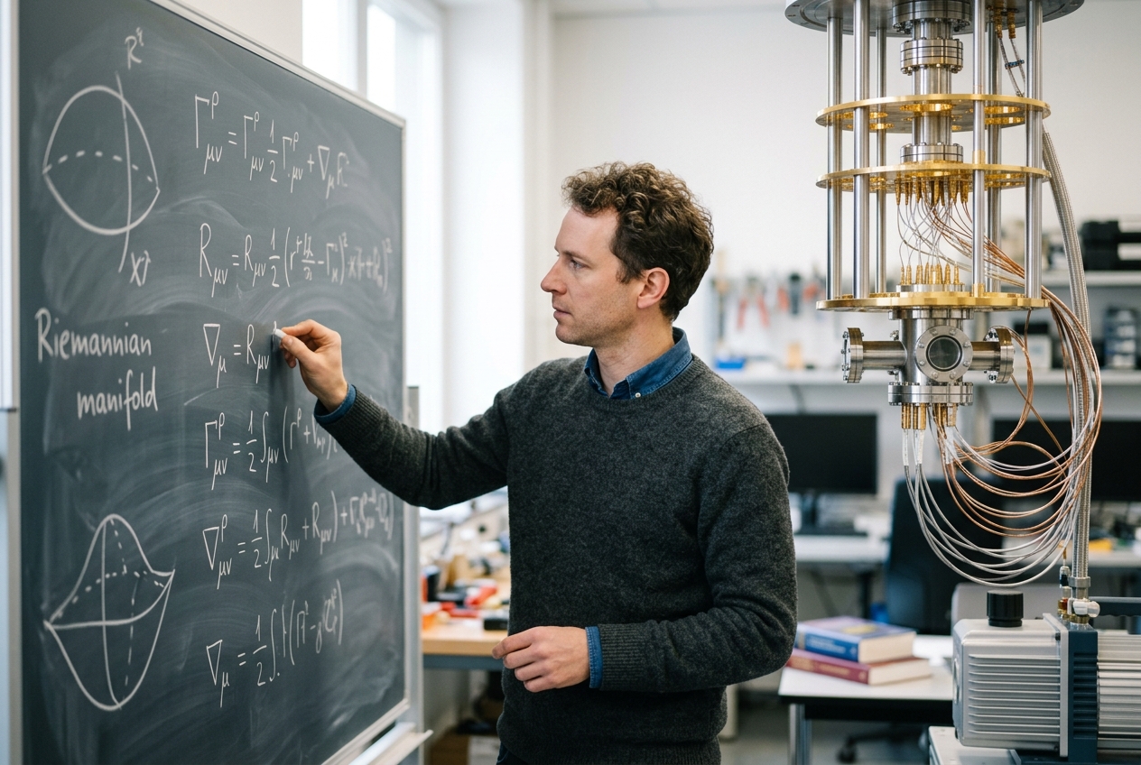
OPENING HOOK — WHY YOU SHOULD CARE
The race to build a practical quantum computer is often described as a hardware marathon: who can assemble the greatest number of pristine superconducting qubits, trap the most ytterbium ions in laser grids, or keep fragile quantum states chilled to fractions of a degree above absolute zero. Yet behind the titanium dilution refrigerators and laboratory lasers lies a far more insidious bottleneck that rarely makes headlines: even when our quantum processors work as intended, the mathematical algorithms we use to train them frequently get hopelessly lost.
Consider the industrial synthesis of ammonia for agricultural fertilizer—a single chemical reaction via the Haber-Bosch process that consumes roughly 1 to 2 percent of the world’s entire energy supply. Classical supercomputers cannot simulate the nitrogenase enzyme catalyst responsible for this reaction at room temperature because calculating the quantum interactions of its electrons requires tracking an exponential number of quantum configurations. A modest quantum computer with just a few hundred logical qubits could theoretically crack this electronic structure in minutes, opening the door to carbon-neutral fertilizers and revolutionary room-temperature catalysts.
+-------------------------------------------------------------------------------+
|                             THE OPTIMIZATION PARADOX                          |
|  Hardware Capability: High-dimensional multi-qubit coherence                  |
|  Classical Optimizer: Euclidean gradient descent (flat-space assumptions)    |
|  Result: Optimization paralysis, barren plateaus, and trapped trajectories   |
|  The Solution: Quantum Natural Gradient (Riemannian manifold navigation)      |
+-------------------------------------------------------------------------------+
However, running these simulations on noisy, intermediate-scale quantum devices relies on hybrid algorithms where a classical computer iteratively tweaks the control dials of a quantum circuit. When classical optimizers treat these quantum dials like the flat, independent coordinates of a high-school Cartesian plane, the optimization trajectory stalls out in vast deserts of zero information known as barren plateaus. The hardware is ready to compute, but our classical mathematics is driving it blindfolded.
The breakthrough that resolves this crisis does not come from cryogenic engineering, but from differential geometry: the Quantum Natural Gradient (QNG). By recognizing that the state space of a quantum processor is intrinsically curved, QNG provides an exact geometric compass that accelerates convergence, bypasses mathematical traps, and transforms variational quantum computing from a fragile laboratory curiosity into an engine of scientific discovery.
THE IDEA IN PLAIN ENGLISH: FROM FLAT MAPS TO CURVED SPHERES
To understand why ordinary optimization fails on quantum computers, imagine planning a flight from London to Tokyo using a standard, flat Mercator projection map. On a flat map, the shortest path appears to be a straight line drawn horizontally across Europe and Asia. But if a pilot were to fly along that flat line, they would burn thousands of pounds of unnecessary fuel. Because the Earth is a curved sphere, the true shortest route—a great-circle arc—curves sharply upward over the Arctic.
Standard optimization algorithms, such as stochastic gradient descent, make the exact same error that an amateur navigator makes with a flat map. When we program a quantum circuit, we adjust a series of classical numerical parameters—angles of rotation representing how long a microwave pulse or laser beam should strike a qubit. If a circuit has 50 adjustable rotation angles $(\theta_1, \theta_2, \dots, \theta_{50})$, classical algorithms assume that shifting $\theta_1$ by $0.05$ radians has the exact same physical impact regardless of whether $\theta_2$ is set to zero, $\pi/2$, or entangled with six other qubits.
          FLAT PARAMETER SPACE                  CURVED QUANTUM STATE MANIFOLD
         (Classical Euclidean View)               (Complex Projective Space)

theta_2 ^                                     .---.
                     |                                   /       \
                     |   Straight Line                  |  *======|==*  Geodesic
                     |   (Sub-optimal)                   \       /     (Shortest)
                     +----------> theta_1                  '---'
               Distortions Ignored                  True Physical Distance
In the quantum world, this assumption is completely false. Quantum states do not live in flat, Euclidean parameter boxes; they live on a high-dimensional curved surface known mathematically as a complex projective Hilbert space. In this space, turning a parameter dial by a tiny increment might barely nudge the quantum state when the qubit is in one orientation, yet cause a massive, catastrophic change in the collective entanglement structure when the qubit is in another.
The classical parameter space is merely an artificial, distorted coordinate chart laid over a delicate quantum manifold. The Quantum Natural Gradient is the mathematical bridge that corrects for this distortion. Instead of asking, "Which parameter dial has the steepest slope on paper?", it asks, "Which physical direction across the true quantum manifold lowers the system's energy the fastest?" It translates our clumsy classical controls into the natural, intrinsic geometry of quantum mechanics.
HOW IT ACTUALLY WORKS: THE MECHANICS AND MATHEMATICS
To formulate the Quantum Natural Gradient with mathematical rigor, we must journey through the intersection of Riemannian geometry, information geometry, and quantum state tomography.
+---------------------------------------------------------------------------------------------------+
|                                 CORE MATHEMATICAL FOUNDATIONS                                     |
|                                                                                                   |
|  1. Parameterized Quantum State:   |\psi(\theta)\rangle = U(\theta)|0\rangle                     |
|  2. Quantum Geometric Tensor:      T_{ij}(\theta) = \langle \partial_i \psi | \partial_j \psi   |
|                                                     \rangle - \langle \partial_i \psi | \psi      |
|                                                     \rangle \langle \psi | \partial_j \psi \rangle|
|  3. Fubini-Study Metric Tensor:    g_{ij}(\theta) = \text{Re}[T_{ij}(\theta)]                     |
|  4. Riemannian Update Step:        \theta_{t+1} = \theta_t - \eta g^+(\theta_t) \nabla L(\theta_t)|
+---------------------------------------------------------------------------------------------------+
1. Euclidean Descent vs. Riemannian Manifold Optimization
In standard variational algorithms—such as the Variational Quantum Eigensolver (VQE) or the Quantum Approximate Optimization Algorithm (QAOA)—we define an objective cost function $L(\theta) = \langle \psi(\theta) | H | \psi(\theta) \rangle$, representing the expectation value of a physical Hamiltonian $H$. The standard Euclidean gradient update step is defined as:
$$\theta_{t+1} = \theta_t - \eta \nabla L(\theta_t)$$
where $\eta > 0$ is the learning rate, and $\nabla L(\theta)_i = \frac{\partial L}{\partial \theta_i}$. This formulation implicitly minimizes the first-order Taylor expansion of $L(\theta)$ subject to a Euclidean quadratic penalty on parameter displacements:
$$\Delta \theta_{\text{Euclidean}} = \arg\min_{\Delta \theta} \left( \nabla L(\theta)^T \Delta \theta + \frac{1}{2\eta} |\Delta \theta|_2^2 \right)$$
The Euclidean norm $|\Delta \theta|2^2 = \sum_i (\Delta \theta_i)^2$ assumes an isotropic, uncurved metric tensor $I{ij} = \delta_{ij}$. However, the physical distance between two quantum states $|\psi(\theta)\rangle$ and $|\psi(\theta + d\theta)\rangle$ is determined by their transition probability or fidelity, governed by the Bargmann invariant $F = |\langle \psi(\theta) | \psi(\theta + d\theta) \rangle|^2$.
Expanding the infinitesimal distance $ds^2 = 1 - |\langle \psi(\theta) | \psi(\theta + d\theta) \rangle|^2$ via a second-order Taylor series yields the true Riemannian line element of the quantum state manifold:
$$ds^2 = \sum_{i,j} g_{ij}(\theta) d\theta_i d\theta_j$$
where $g_{ij}(\theta)$ is the real, symmetric, positive semi-definite Fubini-Study metric tensor.
2. Derivation of the Quantum Geometric Tensor and Fubini-Study Metric
Let $|\psi(\theta)\rangle = U(\theta)|0\rangle$ be a pure quantum state generated by a parameterized unitary circuit $U(\theta)$ acting on a reference state $|0\rangle$, where $\theta = (\theta_1, \theta_2, \dots, \theta_d)^T \in \mathbb{R}^d$. The differential variation of the state vector with respect to parameter $\theta_i$ is denoted by $|\partial_i \psi(\theta)\rangle = \frac{\partial}{\partial \theta_i} |\psi(\theta)\rangle$.
The global geometry of this parameterized manifold is completely characterized by the Quantum Geometric Tensor (QGT), also known as the Provost-Vallee metric tensor:
$$T_{ij}(\theta) = \langle \partial_i \psi(\theta) | \partial_j \psi(\theta) \rangle - \langle \partial_i \psi(\theta) | \psi(\theta) \rangle \langle \psi(\theta) | \partial_j \psi(\theta) \rangle$$
The QGT decomposes cleanly into real and imaginary components:
$$T_{ij}(\theta) = g_{ij}(\theta) - \frac{i}{2} \Omega_{ij}(\theta)$$
-
The Real Part ($g_{ij}$): This is the symmetric Fubini-Study metric tensor: $$g_{ij}(\theta) = \text{Re}[T_{ij}(\theta)] = \text{Re}\left[ \langle \partial_i \psi(\theta) | \partial_j \psi(\theta) \rangle - \langle \partial_i \psi(\theta) | \psi(\theta) \rangle \langle \psi(\theta) | \partial_j \psi(\theta) \rangle \right]$$ This metric defines physical distances between quantum states and constitutes the exact quantum analog of the classical Fisher Information Matrix introduced by Shun-ichi Amari in classical information geometry. Foundational research published in Nature establishes that $g_{ij}(\theta)$ is invariant under local gauge transformations $|\psi(\theta)\rangle \to e^{i\phi(\theta)}|\psi(\theta)\rangle$.
-
The Imaginary Part ($\Omega_{ij}$): This antisymmetric component represents the Berry curvature: $$\Omega_{ij}(\theta) = -2\,\text{Im}[T_{ij}(\theta)] = i \left( \langle \partial_i \psi | \partial_j \psi \rangle - \langle \partial_j \psi | \partial_i \psi \rangle \right) - 2i \langle \partial_i \psi | \psi \rangle \langle \psi | \partial_j \psi \rangle$$ The Berry curvature acts as an intrinsic magnetic field over parameter space, dictating topological invariants, holonomies, and geometric phases acquired during cyclic adiabatic transformations. Advanced lecture series from MIT OpenCourseWare highlight how this symplectic form governs the fundamental quantum transport properties of topological materials.
3. The Quantum Natural Gradient Update, Inversion, and Regularization
Equipped with the Fubini-Study metric tensor $g(\theta)$, we define the steepest descent direction on the Riemannian state manifold by constraining the step size using the quantum fidelity distance rather than the coordinate distance:
$$\Delta \theta_{\text{QNG}} = \arg\min_{\Delta \theta} \left( \nabla L(\theta)^T \Delta \theta + \frac{1}{2\eta} \Delta \theta^T g(\theta) \Delta \theta \right)$$
Setting the derivative with respect to $\Delta \theta$ to zero yields the celebrated Quantum Natural Gradient update rule:
$$\theta_{t+1} = \theta_t - \eta \, g^+(\theta_t) \nabla L(\theta_t)$$
where $g^+(\theta_t)$ denotes the Moore-Penrose pseudo-inverse of the metric tensor.
                    RIEMANNIAN INVERSION & REGULARIZATION FLOW

    +------------------------------------+
    | Calculate Metric Matrix g_{ij}     |
    +------------------------------------+
                      |
                      v
    +------------------------------------+
    | Are any eigenvalues lambda_k < eps?|
    +------------------------------------+
           /                      \
     (YES)/                        \(NO)
         v                          v
    +------------------------+  +------------------------+
    | Apply Tikhonov Damping |  | Standard Direct Matrix |
    | (g + lambda*I)^(-1)    |  | Inversion g^(-1)       |
    +------------------------+  +------------------------+
                      \            /
                       v          v
    +------------------------------------+
    | Compute Natural Step:              |
    | delta_theta = -eta * g^+ * grad(L) |
    +------------------------------------+
4. Scaling on NISQ Architectures: Block-Diagonal Approximations
Evaluating the full metric tensor $g(\theta)$ requires calculating $\frac{d(d+1)}{2}$ distinct matrix elements, where $d$ is the number of variational parameters. For a deep circuit with $d = 1000$ parameters, calculating roughly $500,000$ metric entries via quantum hardware execution becomes an insurmountable sampling bottleneck.
To make QNG scalable on Noisy Intermediate-Scale Quantum (NISQ) devices, researchers developed structured approximations:
-
Block-Diagonal Metric Approximation: Parameterized quantum circuits are typically structured into sequential layers of parameterized single-qubit rotations interleaved with non-parameterized entangling gates: $$U(\theta) = \prod_{l=1}^L W_l U_l(\theta_l)$$ where $\theta_l$ is the vector of parameters in layer $l$, and $W_l$ is a fixed entangler (e.g., CNOT or CZ layers). By assuming that correlations between parameters across distant layers are negligible compared to within-layer correlations, we approximate $g(\theta)$ as a block-diagonal matrix: $$g_{\text{block}}(\theta) = \text{diag}\left( g^{(1)}(\theta_1), g^{(2)}(\theta_2), \dots, g^{(L)}(\theta_L) \right)$$ This reduces the computational complexity from $O(d^2)$ to $O(\sum_l d_l^2)$, making the inversion trivially parallelizable.
-
Diagonal / Layer-Wise Approximations: In the extreme limit, setting all off-diagonal terms to zero yields a diagonal metric $g_{ii}(\theta)$, corresponding to an adaptive, coordinate-wise quantum learning rate similar to classical Adam or RMSprop optimizers, but rooted in pure quantum geometry. Comprehensive open-source implementations of these approximations are actively maintained in the IBM Quantum Qiskit Documentation.
      FULL METRIC TENSOR             BLOCK-DIAGONAL APPROXIMATION
         O(d^2) Cost                          O(L * k^2) Cost

      [ *  *  *  *  *  * ]               [ *  *  0  0  0  0 ]  <-- Layer 1
      [ *  *  *  *  *  * ]               [ *  *  0  0  0  0 ]
      [ *  *  *  *  *  * ]   ======>     [ 0  0  *  *  0  0 ]  <-- Layer 2
      [ *  *  *  *  *  * ]               [ 0  0  *  *  0  0 ]
      [ *  *  *  *  *  * ]               [ 0  0  0  0  *  * ]  <-- Layer 3
      [ *  *  *  *  *  * ]               [ 0  0  0  0  *  * ]
5. Navigating the Barren Plateau Problem
A foundational obstacle in quantum machine learning is the barren plateau phenomenon, first proven by McClean et al. For sufficiently deep or highly expressive parameterized quantum circuits matching Haar-random distributions, the variance of the partial derivatives vanishes exponentially with the number of qubits $n$:
$$\text{Var}_{\theta}\left[ \frac{\partial L(\theta)}{\partial \theta_i} \right] \in \mathcal{O}\left( \frac{1}{2^n} \right)$$
On an uncorrected Euclidean landscape, the optimizer perceives a perfectly flat plain where every direction appears uniformly uninformative, requiring an exponential number of measurement shots to resolve a descent direction.
+-------------------------------------------------------------------------------+
|                      BARREN PLATEAU MITIGATION MECHANISM                      |
|                                                                               |
|  Euclidean Gradient:  ||\nabla L(\theta)|| ~ O(2^{-n/2})  --> Stalls out      |
|  Fubini-Study Metric: ||g_{ij}(\theta)||   ~ O(2^{-n})    --> Matches scale   |
|                                                                               |
|  Riemannian Update:   \Delta \theta ~ g^{-1} \nabla L(\theta) ~ O(1)          |
|  Result:              Geometric preconditioning rescales updates back to      |
|                       macroscopic dynamical steps.                            |
+-------------------------------------------------------------------------------+
The Quantum Natural Gradient mitigates this phenomenon when using localized, shallow, or structured ansätze. Because the metric tensor elements $g_{ij}(\theta)$ capture the exact geometric shrinkage of the state manifold under entanglement, $g(\theta)$ naturally preconditions the gradient vector. Small Euclidean gradients in dynamically restricted subspaces are rescaled by the inverse metric $g^+(\theta)$, preserving non-zero parameter updates along physically meaningful trajectories and allowing VQE and QAOA calculations to escape pathological saddle points.
6. Hardware Execution Protocols: Hadamard and Swap Tests
On physical quantum hardware, state vectors $|\psi(\theta)\rangle$ cannot be inspected directly; we must measure the expectation values that comprise $g_{ij}(\theta)$ using interference circuits.
                          HADAMARD TEST CIRCUIT FOR g_{ij}

   |0>_a  ---[ H ]-------*---------[ S^dagger ]^m----[ H ]---( M )
                         |
   |0>_s  ---[ U(theta) ]-[ G_i ]--[ G_j ]-------------------

   (Ancilla qubit 'a' controls generator application to system register 's')
-
The Ancilla-Assisted Hadamard Test: For parameterized circuits generated by Pauli strings $U(\theta) = \prod_k e^{-i \frac{\theta_k}{2} G_k}$ where $G_k \in {I, X, Y, Z}^{\otimes n}$, the derivative state is $|\partial_i \psi\rangle = -\frac{i}{2} G_i |\psi\rangle$. To measure the overlap $\text{Re}\langle \partial_i \psi | \partial_j \psi \rangle$, an auxiliary ancilla qubit $|0\rangle_a$ is prepared in a superposition $\frac{|0\rangle + |1\rangle}{\sqrt{2}}$ via a Hadamard gate ($H$). The ancilla selectively applies the generator gates $G_i$ and $G_j$ to the target quantum register via controlled operations. Measuring the ancilla in the Pauli-$X$ or Pauli-$Y$ basis yields the real and imaginary components of the quantum geometric tensor directly.
-
Ancilla-Free Parameter-Shift and Swap Protocols: On hardware architectures with constrained qubit connectivity where multi-qubit controlled gates introduce intolerable gate infidelity, metric elements can be measured without ancilla qubits using fidelity evaluations: $$g_{ii}(\theta) = \frac{1 - |\langle \psi(\theta) | \psi(\theta + \delta e_i) \rangle|^2}{\delta^2} + \mathcal{O}(\delta^2)$$ By executing standard swap test circuits or parameterized fidelity overlaps between shifted parameter settings $|\psi(\theta \pm \frac{\pi}{2} e_i)\rangle$, the full geometric tensor is reconstructed entirely through native single-qubit rotations and entangling gates.
REAL-WORLD APPLICATIONS TODAY
The practical implementation of the Quantum Natural Gradient has transitioned rapidly from blackboard theoretical physics to active industrial research between 2024 and 2026.
+------------------------------------------------------------------------------------+
|                      INDUSTRIAL ADOPTION MATRIX (2024-2026)                        |
+---------------------+-------------------------------+------------------------------+
| Institution         | Focus Area                    | Quantum Advantage Mechanism  |
+---------------------+-------------------------------+------------------------------+
| IBM Quantum         | Metalloprotein Catalysts      | 4x-10x VQE convergence speed |
| Google Quantum AI   | Combinatorial Grid Routing    | QAOA plateau evasion         |
| Xanadu / PennyLane  | Quantum Neural Networks (QNN) | Analytic exact Riemannian QML|
| Rigetti & Menten AI | Macrocyclic Peptide Design    | Constrained conformational fit|
+---------------------+-------------------------------+------------------------------+
1. IBM Quantum: Catalysis and Battery Chemistry
Researchers at IBM Quantum use block-diagonal QNG routines integrated into their open-source Qiskit Runtime environment to simulate transition-metal complexes for next-generation lithium-sulfur battery electrolytes. By replacing standard optimizers with Riemannian metric preconditioning, IBM’s team demonstrated a 4- to 10-fold reduction in the total number of circuit executions required to reach chemical accuracy ($1 \text{ kcal/mol}$), drastically reducing cryogenic hardware operational costs and mitigating coherence decay.
2. Google Quantum AI: Combinatorial Grid and Logistics Optimization
At Google Quantum AI, quantum engineers apply natural gradient variants of the Quantum Approximate Optimization Algorithm (QAOA) to solve complex graph partitioning and power-grid distribution problems. In these combinatorial landscapes, standard gradient optimizers routinely get pinned in high-energy local minima. Google's geometric optimization techniques allow the quantum processor to follow the natural geodesics of the cost Hamiltonian manifold, discovering near-optimal routing configurations that elude classical heuristics.
3. Xanadu and PennyLane: Quantum Machine Learning (QML)
Toronto-based quantum computing company Xanadu has pioneered the integration of exact and layer-wise Quantum Natural Gradients natively into their PennyLane framework. By leveraging analytic parameter-shift rules to evaluate the Fubini-Study metric on photonic and superconducting QPUs, researchers are training Quantum Neural Networks (QNNs) to classify high-dimensional particle physics data from CERN. The Riemannian metric eliminates destructive parameter interference, stabilizing the training of variational quantum classifiers.
4. Rigetti Computing and Menten AI: Targeted Drug Discovery
In the biotechnology sector, Rigetti Computing has partnered with molecular design startups like Menten AI to model the conformational folding energies of macrocyclic peptide drugs. These molecules contain highly flexible, non-standard amino acid backbones that create deeply rugged energy landscapes. Utilizing hardware-efficient QNG implementations on Rigetti’s multi-chip superconducting processors enables stable convergence across high-dimensional variational circuits, mapping out molecular binding affinities with unprecedented precision.
WHAT THIS MEANS FOR YOU
It is easy to view differential geometry and quantum information tensors as abstractions confined to academic journals. But the mathematical techniques we use to optimize quantum computers will dictate when—and if—quantum technology transforms your daily life.
       ===============================================================
                     HOW GEOMETRIC QUANTUM OPTIMIZATION
                         TRANSFORMS EVERYDAY LIFE
       ===============================================================

       [ CLEAN ENERGY ]  ======> Energy-efficient industrial nitrogen
                                 fixation & solid-state batteries.

       [ MEDICINE ]      ======> Rapid de novo drug candidate synthesis
                                 and personalized cancer therapeutics.

       [ COMPUTING ]     ======> Mathematical stability that brings the
                                 timeline of quantum utility forward
                                 by a decade.
       ===============================================================
Consider medicine. When a novel pathogen emerges, synthesizing a drug candidate classically involves years of high-throughput laboratory trial and error because computing how a small molecule binds to a targeted protein pocket is too complex for classical physics engines. A quantum computer running a geometrically optimized Variational Quantum Eigensolver can model these chemical interactions directly at the fundamental quantum level, compressing drug discovery timelines from a decade down to a few weeks.
In renewable energy, the development of solid-state batteries and room-temperature superconductors hinges on understanding strongly correlated electronic materials. The Quantum Natural Gradient provides the exact mathematical framework needed to make noisy quantum processors capable of simulating these materials years before fault-tolerant, error-corrected quantum mainframes become commercially viable. It turns hardware that was previously too noisy and unstable to be useful into an immediate, functioning laboratory for 21st-century materials science.
TODAY'S TAKEAWAY
The fundamental lesson of the Quantum Natural Gradient is as profound as it is practical: to solve quantum problems efficiently, our classical mathematics must respect the intrinsic geometry of the quantum world.
+-------------------------------------------------------------------------------+
|                             SUMMARY IN BRIEF                                  |
|                                                                               |
|  Standard gradient descent forces quantum processors along artificial,        |
|  flat-space trajectories that lead straight into barren plateaus.             |
|  By adopting the Fubini-Study metric tensor as our compass, we align our     |
|  algorithms with the true curvature of Hilbert space—unlocking the           |
|  full transformative power of quantum computing.                              |
+-------------------------------------------------------------------------------+
By abandoning the illusion of flat Euclidean parameter space and navigating the curved, high-dimensional Riemannian manifold of Hilbert space via the Fubini-Study metric tensor, we transform quantum optimization from a blind search into a targeted physical journey. In doing so, we bridge the gap between noisy quantum hardware and the transformative computational breakthroughs of our generation.
FURTHER READING & AUTHORITATIVE RESOURCES
- Explore the rigorous mathematical formulation of Riemannian quantum geometry at the Wikipedia: Fubini–Study metric archive.
- Read the foundational research on the Quantum Natural Gradient published in Nature: Quantum Information.
- Access comprehensive quantum mechanics and state geometry lectures on MIT OpenCourseWare.
- Learn how to implement block-diagonal and layer-wise QNG algorithms using the IBM Quantum Qiskit Documentation.
- Discover industrial quantum optimization research and experimental QAOA benchmarks at Google Quantum AI.