Lindblad Master Equation: Modeling Markovian Open Dynamics and Environmental Dissipation in Quantum Systems
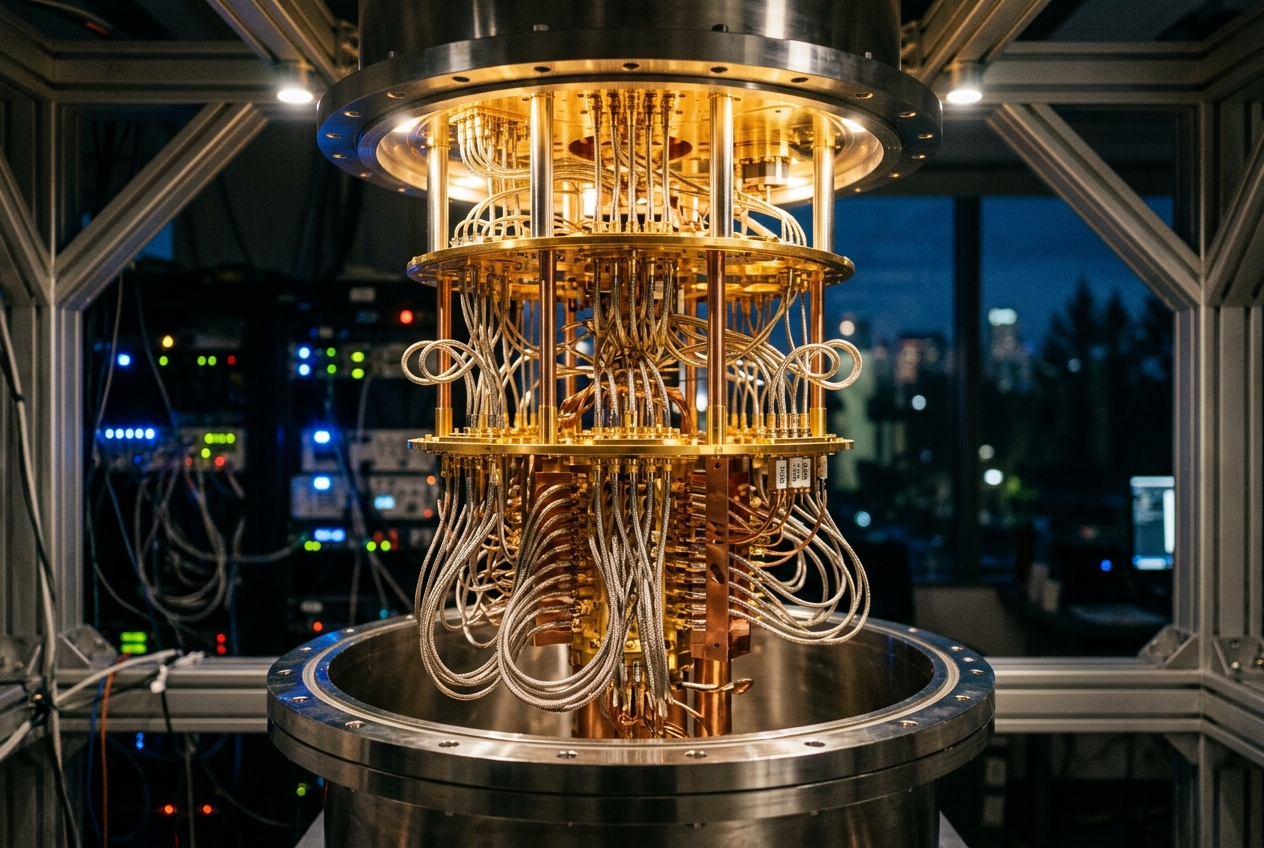
A solitary quantum processor operates at mere millikelvins above absolute zero, shielded inside nested cylinders of gold-plated copper, mu-metal magnetic shielding, and cryopumped vacuum chambers. In spite of this monumental isolation, the outside world invariably seeps in. A stray infrared photon traveling down a coaxial readout cable, a high-energy cosmic ray striking the silicon substrate, or subtle charge fluctuations in nearby dielectric oxides can instantly annihilate a computation.
+-----------------------------------------------------------------------------------+
|                           THE OPEN QUANTUM REALITY                                |
|                                                                                   |
|    CLOSED SYSTEM (IDEAL)                        OPEN SYSTEM (REALITY)             |
|    • Isolated from universe                    • Constantly coupled to bath       |
|    • Reversible unitary evolution (U)          • Irreversible information loss    |
|    • Pure state: |ψ⟩                           • Mixed state: Density Matrix ρ    |
|    • Entropy is zero and constant              • Entropy increases monotonically  |
|    • Governed by: Schrödinger Equation         • Governed by: Lindblad / GKSL     |
+-----------------------------------------------------------------------------------+
When a quantum state interacts with its environment, it does not simply vanish into thin air; rather, its delicate phase coherence bleeds into the trillions of untracked atoms of the surrounding universe. Standard textbook quantum mechanics, governed by the celebrated, reversible Schrödinger equation, is fundamentally powerless to describe this loss.
To calculate how quantum systems decay, dephase, and equilibrate, physicists and engineers must turn to the master equation of open quantum systems: the Gorini-Kossakowski-Sudarshan-Lindblad (GKSL) equation, commonly known as the Lindblad master equation. It is the mathematical bridge connecting the pristine, reversible realm of pure quantum theory to the messy, irreversible, entropy-increasing reality of the physical universe. Without it, the modern quantum computing industry would be designing hardware completely in the dark.
The Idea in Plain English: Escaping the Closed-System Fantasy
To understand why a new mathematical framework is required, consider a classical analogy: a grandfather clock's pendulum swinging in an absolute vacuum on frictionless bearings. Under these pristine, idealized conditions, Newton’s laws of motion predict that the pendulum will oscillate back and forth forever. The system’s total energy is strictly conserved, and its motion is mathematically time-reversible: if you reverse the arrow of time, the equations of motion remain perfectly valid.
Now, place that same pendulum in an ordinary living room. As it swings, it collides with quintillions of nitrogen and oxygen molecules in the air, while its pivots generate microscopic friction against their mounts. With every swing, the pendulum transfers a minute fraction of its kinetic energy and directional momentum into the chaotic thermal motion of the room's atmosphere. Eventually, the pendulum comes to a dead halt.
If your mathematical model only tracks the pendulum's position and velocity while ignoring the surrounding air, energy appears to vanish, and the equations of motion fail to predict reality. You are no longer observing a closed system; you are observing an open system dissipating into an environmental reservoir.
                  +----------------------------------------+
                  |         ENVIRONMENTAL RESERVOIR        |
                  |     (Thermal Bath, Phonons, Photons)   |
                  |                                        |
                  |      ^                          |      |
                  |      | Irreversible             | Back-action / |
                  |      | Information Loss         | Thermal Noise |
                  |      |                          v      |
                  |   +--------------------------------+   |
                  |   |         OPEN QUANTUM           |   |
                  |   |            SYSTEM              |   |
                  |   |   (Qubit / Density Matrix ρ)   |   |
                  |   +--------------------------------+   |
                  +----------------------------------------+
In quantum mechanics, this exact illusion occurs when an experimenter relies exclusively on the Schrödinger equation. The standard wave function, denoted by the ket $|\psi\rangle$, represents a pure state—a condition of complete physical knowledge where quantum superpositions remain mathematically pristine. The time evolution of a pure state is governed by a unitary operator, a mathematical transformation that rigidly preserves total probability (the sum of all probabilities remains precisely 100%) and keeps information strictly conserved. Unitary evolution is completely reversible: running time backwards mathematically recovers the exact initial state.
However, in the real world, no qubit, atom, or molecule is truly isolated. The qubit is constantly bathed in the electromagnetic fluctuations of its wiring, lattice vibrations (phonons) in its substrate, and stray thermal radiation. As the qubit interacts with this colossal reservoir, the system and its environment become inextricably entangled.
Because an experimenter cannot measure or track the countless quantum states of the entire universe, they must mathematically "trace out"—or average over—the environment's degrees of freedom. Once this environmental averaging is performed, the qubit can no longer be described by a single wave function $|\psi\rangle$. It has transitioned into a mixed state, a statistical ensemble of different possible quantum configurations.
To track this mixture of quantum uncertainty and classical probability, physicists replace the state vector with a mathematical object called the density matrix, denoted by the Greek letter $\rho$ (rho). The diagonal elements of this matrix represent the classical probabilities of finding the system in specific energy states (such as the ground state $|0\rangle$ or excited state $|1\rangle$), while the off-diagonal elements—known as quantum coherences—quantify the precise phase relationships that enable quantum superpositions.
Decoherence is the process by which these off-diagonal coherences rapidly decay to zero as phase information leaks into the environmental reservoir, transforming a mysterious quantum superposition into a boring, classical coin-flip distribution. The Lindblad master equation is the exact mathematical engine that tracks the continuous, irreversible trajectory of the density matrix as it undergoes this decay.
How It Actually Works: The Mechanics of the Lindbladian
To describe an open quantum system without tracking every photon in the universe, physicists make three foundational physical assumptions known collectively as the Born-Markov and secular approximations, as thoroughly detailed in educational curricula hosted on MIT OpenCourseWare Quantum Physics.
- The Born Approximation (Weak Coupling): The interaction between the primary quantum system (the qubit) and the environmental reservoir (the thermal bath) is sufficiently weak that the environment is not fundamentally altered by the qubit. The bath acts as an infinite thermodynamic sponge, absorbing entropy without changing its own temperature or structural state.
- The Markov Approximation (Memoryless Bath): The environmental reservoir is so vast and chaotic that any quantum excitation or phase ripple dumped into it by the qubit is dispersed among its infinite degrees of freedom almost instantaneously. The correlation time of the bath is practically zero compared to the timescale of the qubit’s evolution. Consequently, the bath retains no memory of past interactions: what happens to the qubit in the next microsecond depends strictly on its current state, not its historical trajectory.
- The Secular (Rotating-Wave) Approximation: Interactions that oscillate at extremely high frequencies compared to the system's natural decay rate average out to zero over operational timescales and can be safely neglected, ensuring that the resulting mathematical evolution is physically self-consistent.
When these physical conditions are satisfied, the time derivative of the density matrix takes the celebrated continuous form of the Gorini-Kossakowski-Sudarshan-Lindblad (GKSL) master equation:
$$\frac{d\rho}{dt} = -\frac{i}{\hbar}[H, \rho] + \sum_k \left( L_k \rho L_k^\dagger - \frac{1}{2} {L_k^\dagger L_k, \rho} \right)$$
This formula contains two fundamentally distinct dynamical regimes operating simultaneously:
+-----------------------------------------------------------------------------------+
|                        ANATOMY OF THE LINDBLAD MASTER EQUATION                    |
|                                                                                   |
|   dρ/dt  =      - (i/ħ) [H, ρ]          +             D(ρ)                        |
|   ^^^^^         ^^^^^^^^^^^^^^                        ^^^^                        |
|   Rate of       COHERENT DYNAMICS             DISSIPATIVE DYNAMICS (DISSIPATOR)   |
|   Change        • Unitary evolution           • Irreversible decoherence          |
|   of State      • Von Neumann commutator      • Quantum jumps & state decay       |
|                 • Reversible energy shifts    • Preserves CPTP conditions         |
|                                                                                   |
|                 Dissipator Expansion:                                             |
|                 D(ρ) = ∑_k [ L_k ρ L_k†  -  (1/2) { L_k† L_k , ρ } ]             |
|                              ^^^^^^^^^^     ^^^^^^^^^^^^^^^^^^^^^^                |
|                             Quantum Jump     Continuous Non-Unitary               |
|                                "Hits"             Amplitude Decay                 |
+-----------------------------------------------------------------------------------+
1. The Coherent Driver: $- \frac{i}{\hbar}[H, \rho]$
The first term on the right-hand side is the von Neumann commutator, where $H$ is the system's internal Hamiltonian (its energy operator) and $\hbar$ is the reduced Planck constant. The square brackets $[H, \rho] = H\rho - \rho H$ calculate the difference between applying energy transformations before versus after the state. This term represents the pristine, reversible, energy-conserving quantum evolution that the system would undergo if it were entirely isolated from the universe.
2. The Dissipator: $\mathcal{D}(\rho) = \sum_k \left( L_k \rho L_k^\dagger - \frac{1}{2} {L_k^\dagger L_k, \rho} \right)$
The second term is the Lindblad dissipator, the mathematical machine of loss. The curly brackets ${A, B} = AB + BA$ denote an anticommutator. The operators $L_k$ are the crucial Lindblad jump operators (or collapse operators). Each $L_k$ represents a specific, discrete channel through which quantum information or energy is irretrievably dumped into the environment.
The first part of the dissipator, $L_k \rho L_k^\dagger$, describes the discrete "quantum jump" that the system undergoes when an environmental interaction occurs—such as the sudden emission of a microwave photon. The second part, $-\frac{1}{2} {L_k^\dagger L_k, \rho}$, represents the continuous, non-unitary loss of probability amplitude that occurs between jumps.
Remarkably, this anticommutator term can be grouped with the original Hamiltonian to form an effective non-Hermitian Hamiltonian:
$$H_{\text{eff}} = H - \frac{i\hbar}{2}\sum_k L_k^\dagger L_k$$
Under $H_{\text{eff}}$, the quantum state smoothly and deterministically decays in norm, reflecting the increasing probability that a quantum jump will take place as time elapses.
        COHERENT ROTATION                      DISCRETE JUMP / DEPHASING
       (Unitary Hamiltonian)                     (Lindblad Operators L_k)

|0⟩                                         |0⟩
               •                                           •
              / \                                         /
             /   \  [Coherent Rabi                       /   [Spontaneous
            /     \  Oscillations]                      /     T1 Decay:
           /       \                                   /      L = √Γ₁ σ₋]
          v         v                                 v
         |1⟩ <-----> |1⟩                             |1⟩
Complete Positivity: The Bedrock of the GKSL Theorem
Why does the dissipator have this specific mathematical structure? In the mid-1970s, mathematical physicists Vittorio Gorini, Andrzej Kossakowski, George Sudarshan, and independently Göran Lindblad proved a profound theorem published in scientific literature recorded by the American Physical Society / Physical Review.
They proved that if you require a dynamical map to be a continuous Dynamical Semigroup that is both Trace-Preserving (total probability always sums to 1) and Completely Positive (denoted CPTP), the generator must take the GKSL form.
To understand complete positivity, consider a simple positive map that prevents single-qubit probabilities from becoming negative. If you take that qubit and entangle it with a distant, inert spectator qubit that experiences zero noise, an ordinary "positive" mathematical map can inadvertently generate negative probabilities (e.g., a $-20\%$ chance of finding the entangled pair in a particular state). Complete positivity guarantees that no matter how complex the entanglement between the system and any arbitrary ancillary quantum system, all physical probabilities remain strictly non-negative at all times.
The Discrete Alternative: Kraus Operators
While the Lindblad equation describes continuous time evolution using a differential equation, quantum information scientists frequently model noise over discrete intervals (such as across the execution of a single quantum logic gate) using Kraus operators ($M_k$). The Kraus representation models the input-output relationship of a quantum channel:
$$\rho(t) = \sum_k M_k \rho(0) M_k^\dagger, \quad \text{with} \quad \sum_k M_k^\dagger M_k = I$$
Here, $I$ is the identity matrix, ensuring that the trace of the density matrix is conserved. Every Markovian continuous-time Lindblad master equation can be integrated over a finite duration $\Delta t$ to yield an equivalent discrete set of Kraus operators, providing a direct mathematical bridge between differential hardware physics and discrete quantum circuit error analysis, as cataloged in Wikipedia's Gorini–Kossakowski–Sudarshan–Lindblad equation entry.
Physical Realizations: How Qubits Actually Die
To make the Lindblad jump operators concrete, we can examine the specific physical noise mechanisms that degrade modern quantum hardware, such as superconducting circuits and trapped ions.
+-----------------------------------------------------------------------------------+
|                        PHYSICAL NOISE CHANNELS & LINDBLADIANS                     |
|                                                                                   |
|  CHANNEL             JUMP OPERATOR (L_k)        PHYSICAL EFFECT                   |
|  -------------------------------------------------------------------------------  |
|  Energy Relaxation   L₁ = √Γ₁ σ₋                Excited state |1⟩ decays to |0⟩;  |
|  (T1 Decay)                                     Emits a photon into the bath      |
|                                                                                   |
|  Pure Dephasing      L_φ = √(γ_φ / 2) σ_z       Random energy shift; Destroys     |
|  (T2* Noise)                                    phase without losing energy       |
|                                                                                   |
|  Thermal Excitation  L₊ = √Γ₊ σ₊                Absorbs ambient thermal photon;   |
|  (Thermal Bath)                                 Spontaneous excitation |0⟩ to |1⟩ |
+-----------------------------------------------------------------------------------+
1. Energy Relaxation ($T_1$ Decay)
In a superconducting transmon qubit, the excited state $|1\rangle$ sits at a higher microwave energy level than the ground state $|0\rangle$. Over time, the qubit spontaneously drops from $|1\rangle$ to $|0\rangle$ by releasing a microwave photon into the readout resonator or substrate.
This process is modeled by a single Lindblad jump operator proportional to the quantum lowering operator:
$$L_1 = \sqrt{\Gamma_1} \sigma_- = \sqrt{\frac{1}{T_1}} \begin{pmatrix} 0 & 1 \ 0 & 0 \end{pmatrix}$$
Here, $\Gamma_1 = 1/T_1$ is the decay rate, where $T_1$ represents the characteristic longitudinal relaxation time. Inserting $L_1$ into the Lindblad dissipator produces an exponential decay of the excited state population:
$$\rho_{11}(t) = \rho_{11}(0) e^{-t / T_1}$$
     Population / Coherence Decay Over Time
     1.0 |----------------------------------------\
         |                                         \   Energy Relaxation (T1)
     0.8 |                                          \---\
         |     Pure Dephasing (T2)                       \---\
     0.6 |-----\                                              \---\
         |      \                                                  \---\
     0.4 |       \                                                      \---\
         |        \                                                          \
     0.2 |         \                                                          |
         |          \---------------------------------------------------------|
     0.0 +---------------------------------------------------------------------
         0                  Time (Microseconds)                     5 * T1
2. Pure Dephasing ($T_2^*$ Noise)
A qubit can also lose its quantum information without losing any energy at all. In solid-state systems, low-frequency magnetic flux noise or charge noise causes the energy gap between $|0\rangle$ and $|1\rangle$ to fluctuate randomly. This causes the relative quantum phase between $|0\rangle$ and $|1\rangle$ in a superposition $\frac{1}{\sqrt{2}}(|0\rangle + |1\rangle)$ to drift erratically, randomizing its orientation on the equator of the Bloch sphere.
This process is governed by the Pauli-$Z$ jump operator:
$$L_\phi = \sqrt{\frac{\gamma_\phi}{2}} \sigma_z = \sqrt{\frac{\gamma_\phi}{2}} \begin{pmatrix} 1 & 0 \ 0 & -1 \end{pmatrix}$$
This leaves the diagonal populations $\rho_{00}$ and $\rho_{11}$ completely untouched, while driving the off-diagonal quantum coherences to zero at the rate $\Gamma_2 = \frac{1}{T_2} = \frac{1}{2T_1} + \gamma_\phi$. The total dephasing time $T_2$ is fundamentally bounded by the energy relaxation time: $T_2 \le 2T_1$.
3. Thermal Baths and Detailed Balance
At non-zero temperatures ($T > 0$), the environment contains ambient thermal photons. The system can not only decay, but also absorb thermal energy from the reservoir, jumping upward from $|0\rangle$ to $|1\rangle$ via the raising operator $L_+ = \sqrt{\Gamma_+} \sigma_+$.
The ratio of the upward rate $\Gamma_+$ to the downward rate $\Gamma_-$ satisfies the thermodynamic condition of detailed balance:
$$\frac{\Gamma_+}{\Gamma_-} = e^{-\frac{\hbar \omega}{k_B T}}$$
As $t \to \infty$, the Lindblad equation drives the qubit precisely to the classical Boltzmann thermal equilibrium state $\rho_{\text{th}} = \frac{e^{-H / k_B T}}{\text{Tr}(e^{-H / k_B T})}$, proving that the GKSL equation naturally reproduces fundamental thermodynamics.
Computational Strategies: Solving the Lindblad Equation at Scale
Simulating open quantum systems on classical supercomputers is notoriously demanding. If an isolated quantum system has an $N$-dimensional Hilbert space, its state vector $|\psi\rangle$ contains $N$ complex numbers (where $N = 2^n$ for $n$ qubits). However, its density matrix $\rho$ is an $N \times N$ operator containing $N^2$ complex entries. For a 30-qubit processor, $N \approx 10^9$, which means the density matrix contains $N^2 \approx 10^{18}$ numbers—demanding exabytes of memory just to store a single time slice.
+-----------------------------------------------------------------------------------+
|               DENSITY MATRIX INTEGRATION vs. QUANTUM TRAJECTORIES                 |
|                                                                                   |
|   DIRECT DENSITY MATRIX (ODE)               MONTE CARLO TRAJECTORIES (MCWF)       |
|   • Tracks full ensemble ρ                  • Tracks single wave function |ψ(t)⟩  |
|   • Memory footprint: O(N²)                 • Memory footprint: O(N)              |
|   • Deterministic differential solver       • Stochastic simulation averaged over |
|   • Infeasible for > 15 qubits                thousands of parallel runs          |
|                                             • Scales to 30+ qubits on clusters    |
+-----------------------------------------------------------------------------------+
To circumvent this computational wall, quantum physicists developed the Monte Carlo Wavefunction (MCWF) method, also known as the quantum trajectory method. Instead of propagating the massive $N \times N$ density matrix deterministically, the computer simulates the evolution of an $N$-dimensional pure state wave function $|\psi(t)\rangle$ subject to stochastic (random) quantum jumps:
$$|\psi(t+dt)\rangle = \frac{(I - \frac{i}{\hbar}H_{\text{eff}}dt)|\psi(t)\rangle}{| (I - \frac{i}{\hbar}H_{\text{eff}}dt)|\psi(t)\rangle |}$$
                A Single Stochastic Quantum Trajectory (MCWF)

  |ψ|² Norm
   1.0 |-------\
       |        \--- Continuous non-unitary decay under H_eff
       |             (No jump detected by environmental monitor)
   0.9 |              \
       |               \       * QUANTUM JUMP OCCURS! *
   0.8 |                \      State collapses: |ψ⟩ -> L_k |ψ⟩ / || L_k |ψ⟩ ||
       |                 \     Norm resets instantly to 1.0
   0.0 +------------------+----+---------------------------------------------> Time
                          t*
During each infinitesimal time step $dt$, the algorithm calculates the jump probability $\delta p = \sum_k \langle \psi(t) | L_k^\dagger L_k | \psi(t) \rangle dt$. A pseudo-random number $r \in [0, 1)$ is generated: - If $r > \delta p$, no jump occurs. The state evolves smoothly under the effective non-Hermitian Hamiltonian $H_{\text{eff}}$ and is continuously renormalized. - If $r \le \delta p$, a discrete quantum jump occurs! The state collapses abruptly: $|\psi(t+dt)\rangle = \frac{L_k |\psi(t)\rangle}{\sqrt{\langle \psi | L_k^\dagger L_k | \psi \rangle}}$.
By averaging hundreds or thousands of these individual, randomly generated trajectories, the exact density matrix is reconstructed: $\rho(t) = \mathbb{E}[|\psi(t)\rangle \langle \psi(t)|]$. Because this method only stores $N$-dimensional vectors, it dramatically lowers memory requirements from $O(N^2)$ to $O(N)$, enabling the simulation of realistic open quantum systems across dozens of coupled qubits on high-performance computing clusters.
Real-World Applications Today (2024–2026)
Far from being an abstract exercise in functional analysis, the Lindblad master equation is an indispensable engineering tool across cutting-edge quantum technology sectors.
+------------------------------------------------------------------------------------+
|                         ACTIVE INDUSTRIAL APPLICATIONS                             |
|                                                                                    |
|  SECTOR               LEAD ORGANIZATIONS         APPLICATION FOCUS                 |
|  --------------------------------------------------------------------------------  |
|  Superconducting QPU  IBM Quantum,               Pulse-level optimal control       |
|  Engineering          Google Quantum AI          (GRAPE/DRAG) to suppress leakage  |
|                                                                                    |
|  Fault-Tolerant       Quantinuum, QuEra,         Simulating continuous syndrome    |
|  Error Correction     Amazon Braket              extraction in topological codes   |
|                                                                                    |
|  Nanoscale Sensing    Q-CTRL, Harvard/MIT        Mitigating dephasing in diamond   |
|  & Metrology          Quantum Laboratories       NV-centers for sub-cellular bio   |
|                                                                                    |
|  Light-Harvesting     European Quantum Flagship, Simulating noise-assisted exciton |
|  Quantum Biology      Academic Consortia         energy transport in photosynthesis|
+------------------------------------------------------------------------------------+
1. Pulse-Level Optimal Control in Superconducting Quantum Hardware
At IBM Quantum and Google Quantum AI, hardware engineers program microwave control lines to execute quantum logic gates on superconducting transmon processors. When a transmon qubit is driven with microwave pulses, leakage to non-computational higher energy states (such as the $|2\rangle$ state) and stray electromagnetic crosstalk degrade gate fidelity.
Engineers use open-source numerical packages like QuTiP and Qiskit Dynamics—documented comprehensively on the IBM Quantum / Qiskit Documentation Hub—to integrate the Lindblad equation directly.
By applying numerical optimal control algorithms, such as GRadient Ascent Pulse Engineering (GRAPE) and Derivative Removal by Adiabatic Gate (DRAG), they design pulse envelopes that continuously steer the qubit around environmental dissipation channels, pushing two-qubit gate fidelities past the critical $99.9\%$ threshold.
2. Quantum Error Correction (QEC) and Fault-Tolerant Architectures
Companies like Quantinuum (using trapped ytterbium ions) and QuEra Computing (using neutral rubidium atom arrays) are demonstrating fault-tolerant logical qubits. In quantum error correction, ancilla qubits continuously measure parity syndromes to detect and correct errors without measuring—and thus collapsing—the encoded logical state.
Engineers rely on Lindbladian master equations to model the continuous interaction between physical qubits and their control noise during syndrome measurement cycles. This allows them to benchmark the performance of the surface code and novel bivariate bicycle codes under realistic, asymmetric noise, identifying exact fault-tolerance thresholds before fabricating hardware.
                      SURFACE CODE STABILIZER CYCLE
           Physical Qubit                   Physical Qubit
                (Data)                           (Data)
                  O ------------------------------- O
                  |                                 |
                  |         ANCILLA QUBIT           |
                  |         (Syndrome Check)        |
                  |                 X               |
                  |          [Lindbladian           |
                  |           Noise Model]          |
                  |                                 |
                  O ------------------------------- O
           Physical Qubit                   Physical Qubit
                (Data)                           (Data)
3. Nanoscale Biosensing with Diamond Nitrogen-Vacancy (NV) Centers
In quantum metrology, startups like Q-CTRL and academic research groups design quantum sensors based on nitrogen-vacancy (NV) defect centers in diamond lattices. An NV center acts as an atomic-scale magnetic sensor capable of operating inside living biological cells.
Because the spin of the NV center is exceptionally sensitive to magnetic fluctuations, its pure dephasing rate ($\gamma_\phi$) increases in the presence of external magnetic fields. Researchers invert the Lindblad equation: by measuring the precise decay rate of quantum coherence in the NV center, they reconstruct the magnetic signatures of single neuronal action potentials and map ferritin protein distributions with sub-nanometer spatial resolution.
4. Quantum Biology and Artificial Light-Harvesting
In biophysics, researchers investigating the Fenna-Matthews-Olson (FMO) pigment-protein complex found in green sulfur bacteria utilize the Lindblad equation to study how photosynthetic complexes transfer solar energy with near $100\%$ quantum efficiency.
Published studies in high-impact journals like Nature demonstrate a phenomenon known as Environment-Assisted Quantum Transport (ENAQT). Pure, isolated quantum evolution causes excitons (energy packets) to become trapped in localized destructive interference patterns.
By modeling the system with a Lindbladian thermal bath, biophysicists proved that environmental decoherence de-tunes these destructive traps, allowing energy to diffuse smoothly across chromophores to the chemical reaction center. Engineers are now using these Lindblad-derived biological insights to design biomimetic solar cells with vastly superior light-collection properties.
What This Means for You
It is easy to view the mathematics of open quantum systems as an esoteric concern confined to cleanrooms and supercomputing centers. But the physics modeled by the Lindblad equation will directly shape key technological breakthroughs over the coming decades.
                       HOW DECOHERENCE IMPACTS SOCIETY

    PHARMACEUTICALS               DATA SECURITY               ENERGY STORAGE
          & BIO                  & CYBERSECURITY                & MATERIALS
            |                           |                            |
            v                           v                            v
   Simulation of enzyme        Exact timelines for          Discovery of solid-state
   active sites (FeMoco)       RSA migration to Post-       electrolytes & Room-Temp
   without noise-induced       Quantum Cryptography         Superconductors modeled
   algorithmic collapse.       (NIST Standards).            via open master equations.
1. Unlocking Life-Saving Medicine and Green Chemistry
The primary industrial motivation for building a fault-tolerant quantum computer is simulating molecular chemistry that completely baffles classical supercomputers. Consider the Haber-Bosch process, which consumes roughly $1–2\%$ of the world’s total energy supply to synthesize ammonia for agricultural fertilizer. Soil bacteria perform this exact reaction at room temperature using an enzyme called nitrogenase (specifically the iron-molybdenum cofactor, FeMoco).
Classical supercomputers cannot model the complex, strongly correlated quantum electron clouds of FeMoco. A quantum computer could solve this active site in days—provided its qubits do not succumb to environmental noise before the calculation concludes. Understanding and mitigating Lindbladian dissipation is the single technological prerequisite for designing synthetic, room-temperature catalysts that could eliminate millions of tons of global carbon emissions.
2. The Timeline for Global Cybersecurity
Every time you send a message, access online banking, or store data in the cloud, your privacy is safeguarded by public-key encryption (such as RSA and Elliptic Curve Cryptography). A sufficiently large quantum computer running Shor's algorithm could crack these protocols.
However, because the Lindblad equation models how real physical noise limits gate execution speeds and circuit depths, it provides intelligence agencies and cybersecurity standard bodies (like NIST) with the exact mathematical tools needed to calculate when a fault-tolerant quantum computer will actually arrive. This realistic timeline gives institutions the runway to transition our global financial architecture to Post-Quantum Cryptography (PQC) before catastrophic security breaches occur.
Today's Takeaway
+------------------------------------------------------------------------------------+
|                                 CORE TAKEAWAY                                      |
|                                                                                    |
|   The universe is neither purely isolated nor entirely classical; it is a          |
|   continuous, dynamical exchange of information across quantum boundaries.         |
|   The Lindblad master equation (GKSL theorem) is the definitive mathematical       |
|   architecture of that exchange. It captures the decay of energy (T1), the loss   |
|   of phase coherence (T2), and the emergence of classical thermodynamics from      |
|   pure quantum superposition. To master the quantum future, one must first master  |
|   the mathematics of loss.                                                         |
+------------------------------------------------------------------------------------+