Kochen-Specker Theorem: Refuting Non-Contextual Realism and Establishing Quantum Contextuality
The philosophical foundation of classical physics rests upon the doctrine of non-contextual realism: the ontological assumption that physical systems possess intrinsic, determinate properties that exist independently of observation. Under this classical worldview, a measurement does not create a value; rather, it passively reveals a pre-existing element of physical reality. If one measures the momentum of a billiard ball, the outcome is understood to have been encoded in the ball’s phase space trajectory prior to the interaction with the measuring apparatus. Furthermore, classical measurement is non-contextual: the value revealed for an observable $A$ is strictly invariant whether $A$ is measured alongside a compatible observable $B$ or an alternative compatible observable $C$.
Quantum mechanics delivers a definitive algebraic rejection of this worldview. While Bell's Theorem established that no local hidden-variable theory can reproduce the statistical predictions of quantum mechanics for spatially separated entangled systems, the Kochen-Specker (KS) theorem (proven by Simon Kochen and Ernst Specker in 1967) demonstrates an even more radical, structural feature of quantum theory.
The Kochen-Specker theorem asserts that non-contextual hidden-variable (NCHV) theories are mathematically incompatible with the Hilbert space structure of quantum mechanics for any single quantum system of dimension $d \ge 3$.
Unlike Bell's theorem, the KS theorem: 1. Does not require entanglement: It applies directly to isolated, individual quantum systems (such as a single qutrit or a pair of qubits). 2. Does not rely on spatial separation: It does not invoke relativistic locality or spacelike separation to rule out hidden variables. 3. Is state-independent: The contradiction arises from the non-commutative geometric arrangement of projection operators on the Hilbert space $\mathcal{H}$, meaning that no quantum state—pure or mixed—can admit a non-contextual valuation.
The conceptual precursor to the KS theorem is Andrew Gleason's 1957 Theorem, which characterized probability measures on the lattice of closed subspaces of a Hilbert space. Gleason proved that for $\dim(\mathcal{H}) \ge 3$, every continuous probability measure $P$ on the projection lattice $\mathcal{P}(\mathcal{H})$ can be uniquely represented by a density operator $\rho$ such that $P(E) = \operatorname{Tr}(\rho E)$ for every projection $E \in \mathcal{P}(\mathcal{H})$.
A critical corollary of Gleason's theorem is the non-existence of two-valued dispersion-free measures: there is no measure on $\mathcal{P}(\mathcal{H})$ that maps every projection operator exclusively to the binary truth values ${0, 1}$ while respecting the additivity of probabilities across mutually orthogonal subspaces.
While Gleason’s analytical proof relied on continuous measures and topological properties of the unit sphere, Kochen and Specker constructed a finite, purely combinatorial, and constructive refutation of non-contextuality.
2. Formal Mathematical Statement & The Colorability Problem
To formulate the Kochen-Specker theorem rigorously, let $\mathcal{H}$ be a complex (or real) Hilbert space of finite dimension $d \ge 3$. Let $\mathcal{P}(\mathcal{H})$ denote the set of self-adjoint projection operators on $\mathcal{H}$, where each projector $P$ corresponds to an orthogonal projection onto a one-dimensional ray (subspace) spanned by a unit vector $|\psi\rangle$, denoted $P = |\psi\rangle\langle\psi|$.
The Non-Contextual Valuation Function
An NCHV model posits the existence of a global valuation map:
$$v: \mathcal{P}(\mathcal{H}) \to {0, 1}$$
which assigns a deterministic truth value (1 representing "true" or "system possesses the property", and 0 representing "false") to every projection operator prior to measurement. For this valuation to be physically consistent and non-contextual, it must satisfy two axiomatic constraints:
- Normalization: For the identity operator $\mathbb{I}$, $v(\mathbb{I}) = 1$.
- Sum Rule (Exclusivity & Completeness): For any complete set of mutually orthogonal one-dimensional projectors ${P_i}_{i=1}^d$ satisfying:
$$\sum_{i=1}^d P_i = \mathbb{I} \quad \text{and} \quad P_i P_j = \delta_{ij} P_i$$
the valuation function must assign the value $1$ to exactly one projector and $0$ to all others:
$$\sum_{i=1}^d v(P_i) = 1, \quad \text{where } v(P_i) \in {0, 1}$$
In the language of observables, if a set of mutually commuting operators ${A, B, C, \dots}$ forms a maximal commuting set (a context), their joint measurement is equivalent to measuring a non-degenerate basis of projection operators. Non-contextuality demands that the value $v(P_i)$ assigned to $P_i$ remains identical regardless of which orthogonal basis (measurement context) contains $P_i$.
The Uncolorability Problem on Orthogonality Graphs
The Kochen-Specker theorem can be translated into a graph coloring problem.
Let $G = (V, E)$ be an orthogonality graph embedded in the projective space $\mathbb{CP}^{d-1}$ (or $\mathbb{RP}^{d-1}$): - Vertices ($V$): Represent a finite collection of one-dimensional rays (unit vectors $|\psi_i\rangle$). - Edges ($E$): Connect pairs of vertices $(|\psi_i\rangle, |\psi_j\rangle)$ that are mutually orthogonal ($\langle\psi_i | \psi_j\rangle = 0$).
A complete orthonormal basis of dimension $d$ manifests in $G$ as a clique of size $d$ ($d$-clique). The KS valuation criteria impose the following graph coloring rule:
The KS 1-0 Coloring Rule: Can one assign a binary color $c(v) \in {0, 1}$ to every vertex $v \in V$ such that: 1. No two adjacent vertices both receive the color $1$ (i.e., $(u, v) \in E \implies c(u) \cdot c(v) = 0$). 2. In every maximal $d$-clique $C \subseteq V$, exactly one vertex receives the color $1$ ($\sum_{v \in C} c(v) = 1$).
The Kochen-Specker theorem proves that there exist finite sets of rays in $\mathbb{R}^d$ or $\mathbb{C}^d$ ($d \ge 3$) whose hypergraph of orthogonality cliques admits no valid KS 1-0 coloring.
The obstruction is topological and algebraic: the interlocking structure of shared vertices across multiple measurement bases creates an over-constrained system of linear Diophantine equations over ${0, 1}$ with no simultaneous solution.
3. Canonical Geometric Proofs & Ray Configurations
Historical Evolution: From 117 to 31 Rays
The original 1967 proof by Simon Kochen and Ernst Specker constructed a geometric configuration of 117 rays in the 3-dimensional real Hilbert space $\mathbb{R}^3$. Their construction leveraged geometric projections of points on the unit sphere connected via a complex network of 2D triangles and orthogonality circles, establishing a configuration of interlocking orthogonal triads that admitted no binary valuation.
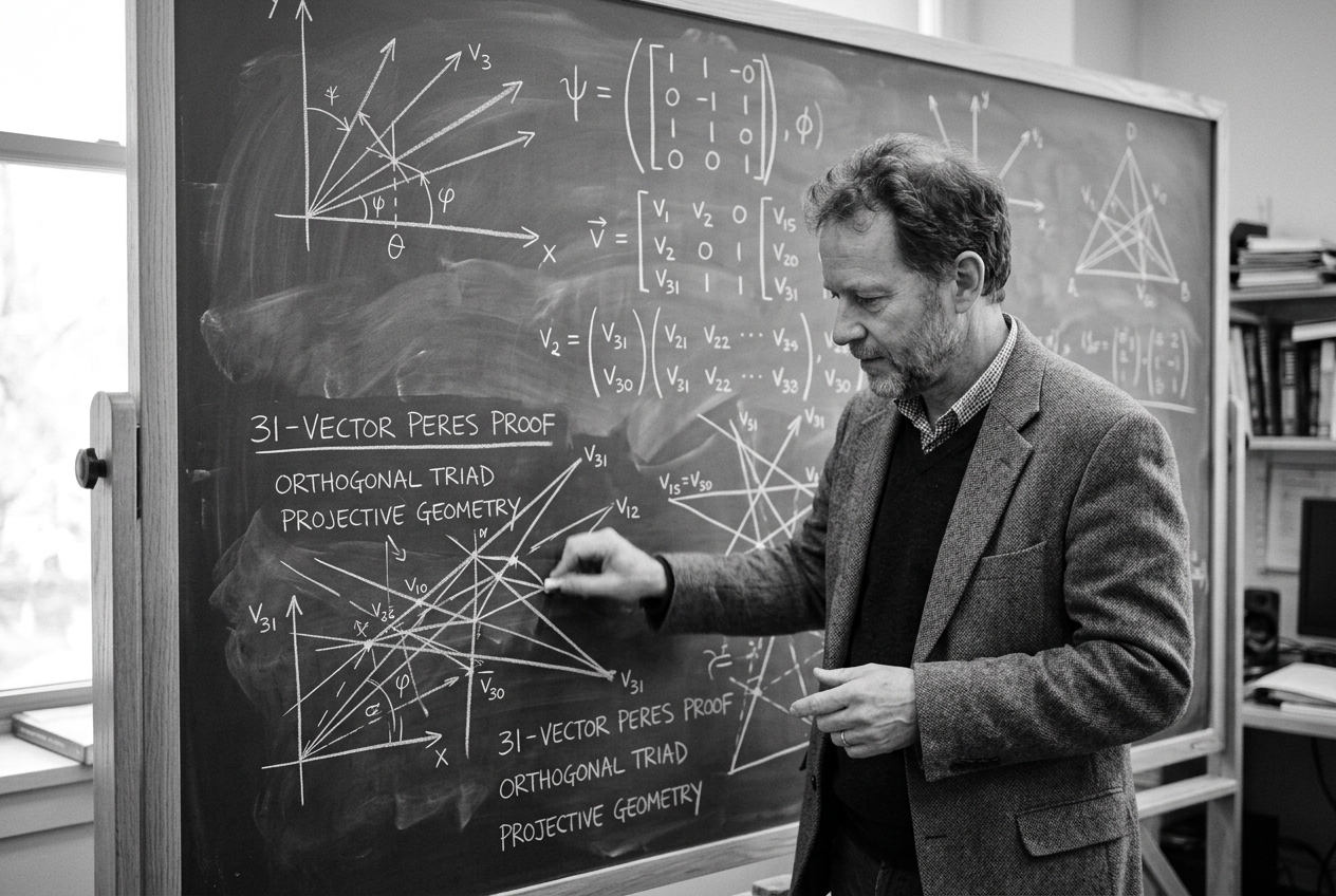
In 1991, Asher Peres streamlined the geometric configuration in $\mathbb{R}^3$: - Peres’s 33-Vector Configuration: Derived from the symmetry groups of the cube and octahedron, utilizing directional rays with coordinate entries chosen from the unnormalized set ${0, \pm 1, \pm \sqrt{2}}$. - Peres’s 31-Vector Configuration: Further reduced the system by projecting vertices along the diagonals and faces of a hypercube, establishing an uncolorable set of 31 rays grouped into 16 interlocking orthogonal bases.
Cabello’s 18-Vector Proof in Dimension $d = 4$
The most mathematically compact and elegant ray-based proof of the Kochen-Specker theorem was formulated by Adán Cabello in 1996 for a 4-dimensional Hilbert space $\mathcal{H} = \mathbb{C}^4$ (isomorphic to a two-qubit state space). Cabello's proof requires only 18 unnormalized rays grouped into 9 complete orthonormal contexts (bases of 4 rays each).
Let the 18 rays $v_1, v_2, \dots, v_{18} \in \mathbb{R}^4$ be defined as follows:
| Ray Identifier | Vector Coordinates $(x_1, x_2, x_3, x_4)^T$ |
|---|---|
| $\mathbf{r}_1$ | $(0, 0, 0, 1)$ |
| $\mathbf{r}_2$ | $(0, 0, 1, 0)$ |
| $\mathbf{r}_3$ | $(1, 1, 0, 0)$ |
| $\mathbf{r}_4$ | $(1, -1, 0, 0)$ |
| $\mathbf{r}_5$ | $(0, 1, 0, 0)$ |
| $\mathbf{r}_6$ | $(1, 0, 1, 0)$ |
| $\mathbf{r}_7$ | $(1, 0, -1, 0)$ |
| $\mathbf{r}_8$ | $(0, 1, 0, 1)$ |
| $\mathbf{r}_9$ | $(1, 0, 0, -1)$ |
| $\mathbf{r}_{10}$ | $(1, -1, -1, 1)$ |
| $\mathbf{r}_{11}$ | $(1, 1, 1, 1)$ |
| $\mathbf{r}_{12}$ | $(0, 0, 1, 1)$ |
| $\mathbf{r}_{13}$ | $(1, 1, 0, -1)$ |
| $\mathbf{r}_{14}$ | $(1, -1, 1, 0)$ |
| $\mathbf{r}_{15}$ | $(1, 1, -1, 0)$ |
| $\mathbf{r}_{16}$ | $(0, 1, 1, 0)$ |
| $\mathbf{r}_{17}$ | $(1, 0, 0, 1)$ |
| $\mathbf{r}_{18}$ | $(1, -1, 0, 1)$ |
These 18 rays form exactly 9 complete orthonormal bases ($B_1$ through $B_9$), where each basis contains 4 mutually orthogonal rays:
- $B_1 = {\mathbf{r}_1, \mathbf{r}_2, \mathbf{r}_3, \mathbf{r}_4}$
- $B_2 = {\mathbf{r}_1, \mathbf{r}_5, \mathbf{r}_6, \mathbf{r}_7}$
- $B_3 = {\mathbf{r}_2, \mathbf{r}_5, \mathbf{r}_8, \mathbf{r}_9}$
- $B_4 = {\mathbf{r}3, \mathbf{r}_8, \mathbf{r}{10}, \mathbf{r}_{11}}$
- $B_5 = {\mathbf{r}4, \mathbf{r}_6, \mathbf{r}{12}, \mathbf{r}_{13}}$
- $B_6 = {\mathbf{r}7, \mathbf{r}_9, \mathbf{r}{14}, \mathbf{r}_{15}}$
- $B_7 = {\mathbf{r}{10}, \mathbf{r}{13}, \mathbf{r}{16}, \mathbf{r}{17}}$
- $B_8 = {\mathbf{r}{11}, \mathbf{r}{12}, \mathbf{r}{16}, \mathbf{r}{18}}$
- $B_9 = {\mathbf{r}{14}, \mathbf{r}{15}, \mathbf{r}{17}, \mathbf{r}{18}}$
The Parity Proof of Contradiction
The contradiction is established via a simple parity counting argument:
- Sum over contexts: According to the KS sum rule, the sum of valuations across the 4 rays of any complete orthonormal basis must equal 1:
$$\sum_{\mathbf{r} \in B_k} v(\mathbf{r}) = 1 \quad \forall k \in {1, 2, \dots, 9}$$
- Summing all 9 contexts: Summing this relation across all 9 bases yields:
$$\sum_{k=1}^9 \sum_{\mathbf{r} \in B_k} v(\mathbf{r}) = \sum_{k=1}^9 1 = 9$$
- Vertex incidence: Crucially, every single ray $\mathbf{r}_i$ ($i \in {1, \dots, 18}$) appears in exactly two distinct bases. Therefore, when expanding the left-hand sum, each valuation $v(\mathbf{r}_i)$ is counted exactly twice:
$$\sum_{k=1}^9 \sum_{\mathbf{r} \in B_k} v(\mathbf{r}) = 2 \sum_{i=1}^{18} v(\mathbf{r}_i)$$
- The Parity Contradiction: Equating the two evaluations:
$$2 \sum_{i=1}^{18} v(\mathbf{r}i) = 9 \implies \sum{i=1}^{18} v(\mathbf{r}_i) = \frac{9}{2}$$
Because $v(\mathbf{r}i) \in {0, 1}$, the sum $\sum{i=1}^{18} v(\mathbf{r}_i)$ must be a non-negative integer, and $2 \sum v(\mathbf{r}_i)$ must be an even integer. However, 9 is an odd integer.
An even number cannot equal an odd number. Hence, no non-contextual valuation $v$ can exist.
The Peres-Mermin Magic Square
While ray-based proofs employ projection operators, Asher Peres and David Mermin formulated an algebraic, operator-based proof of contextuality using the Pauli group for two qubits ($\mathcal{H} = \mathbb{C}^2 \otimes \mathbb{C}^2$, $d = 4$).
Consider the following $3 \times 3$ grid of self-adjoint observables constructed from tensor products of single-qubit Pauli matrices ${\sigma_x, \sigma_y, \sigma_z}$ and the identity $\mathbb{I}$:
Algebraic Properties of the Grid:
- Mutual Commutation: The three operators within every row commute with one another.
- Mutual Commutation: The three operators within every column commute with one another.
- Row Products: Multiplying the operators across each row yields the identity operator $+\mathbb{I}$:
- Row 1: $(\sigma_x \otimes \mathbb{I})(\mathbb{I} \otimes \sigma_x)(\sigma_x \otimes \sigma_x) = \sigma_x^2 \otimes \sigma_x^2 = \mathbb{I} \otimes \mathbb{I} = +\mathbb{I}$
- Row 2: $(\mathbb{I} \otimes \sigma_y)(\sigma_y \otimes \mathbb{I})(\sigma_y \otimes \sigma_y) = \sigma_y^2 \otimes \sigma_y^2 = \mathbb{I} \otimes \mathbb{I} = +\mathbb{I}$
- Row 3: $(\sigma_x \otimes \sigma_y)(\sigma_y \otimes \sigma_x)(\sigma_z \otimes \sigma_z) = (\sigma_x \sigma_y \sigma_z) \otimes (\sigma_y \sigma_x \sigma_z) = (i\sigma_z \sigma_z) \otimes (-i\sigma_z \sigma_z) = i(-i)(\mathbb{I} \otimes \mathbb{I}) = +\mathbb{I}$
- Column Products: Multiplying the operators down columns 1 and 2 yields $+\mathbb{I}$, but column 3 yields $-\mathbb{I}$:
- Column 1: $(\sigma_x \otimes \mathbb{I})(\mathbb{I} \otimes \sigma_y)(\sigma_x \otimes \sigma_y) = \sigma_x^2 \otimes \sigma_y^2 = +\mathbb{I}$
- Column 2: $(\mathbb{I} \otimes \sigma_x)(\sigma_y \otimes \mathbb{I})(\sigma_y \otimes \sigma_x) = \sigma_y^2 \otimes \sigma_x^2 = +\mathbb{I}$
- Column 3: $(\sigma_x \otimes \sigma_x)(\sigma_y \otimes \sigma_y)(\sigma_z \otimes \sigma_z) = (\sigma_x \sigma_y \sigma_z) \otimes (\sigma_x \sigma_y \sigma_z) = (i\mathbb{I}) \otimes (i\mathbb{I}) = i^2 (\mathbb{I} \otimes \mathbb{I}) = -\mathbb{I}$
The Non-Contextual Algebraic Collapse
In an NCHV theory, each observable $A_{ij}$ in the grid possesses a pre-existing scalar measurement outcome $v(A_{ij}) \in {+1, -1}$ (since the eigenvalues of all operators in the square are $\pm 1$). Because the valuation map must preserve functional relations among mutually commuting observables:
$$v(A B) = v(A) v(B) \quad \text{for } [A, B] = 0$$
The product of valuations across the rows and columns must reflect their algebraic products: - For Row 1: $v(A_{11}) v(A_{12}) v(A_{13}) = v(+\mathbb{I}) = +1$ - For Row 2: $v(A_{21}) v(A_{22}) v(A_{23}) = v(+\mathbb{I}) = +1$ - For Row 3: $v(A_{31}) v(A_{32}) v(A_{33}) = v(+\mathbb{I}) = +1$ - For Col 1: $v(A_{11}) v(A_{21}) v(A_{31}) = v(+\mathbb{I}) = +1$ - For Col 2: $v(A_{12}) v(A_{22}) v(A_{32}) = v(+\mathbb{I}) = +1$ - For Col 3: $v(A_{13}) v(A_{23}) v(A_{33}) = v(-\mathbb{I}) = -1$
Let us compute the grand product $M$ of all 9 assigned values:
Taking the product of all three rows:
$$M = \prod_{i=1}^3 \left( \prod_{j=1}^3 v(A_{ij}) \right) = (+1)(+1)(+1) = +1$$
Taking the product of all three columns:
$$M = \prod_{j=1}^3 \left( \prod_{i=1}^3 v(A_{ij}) \right) = (+1)(+1)(-1) = -1$$
Since multiplication over $\mathbb{R}$ is commutative, the grand product of all 9 elements must evaluate to the same value regardless of the order of multiplication. Thus, we arrive at the impossible condition:
$$+1 = -1$$
This operator-level contradiction proves that no classical non-contextual assignment of eigenvalues can reproduce the algebraic structure of commuting quantum observables.
4. Experimental Verifications & Operational Contextuality
To transition the Kochen-Specker theorem from a structural "no-go" proof to an empirical test in the laboratory, one must formulate operational, statistical contextuality inequalities analogous to the Clauser-Horne-Shimony-Holt (CHSH) formulation of Bell's theorem.
The Cabello-Severini-Winter (CSW) Graph-Theoretic Framework
In 2014, Adán Cabello, Simone Severini, and Andreas Winter established the foundational CSW framework, unifying all non-contextuality inequalities and Bell inequalities through graph theory.
Let $G = (V, E)$ be an exclusivity graph where vertices represent measurement events (projectors $P_i$) and edges represent mutual exclusivity ($P_i P_j = 0$). For any state $|\psi\rangle$, the sum of probabilities of these events is bounded by three fundamental graph invariants:
- Classical (Non-Contextual) Bound: Governed by the independence number $\alpha(G)$ of the graph (the size of the largest set of mutually non-adjacent vertices):
$$\sum_{i \in V} P(v_i) \le \alpha(G)$$
- Quantum Bound: Governed by the Lovász theta function $\vartheta(G)$ of the graph:
$$\sum_{i \in V} P(v_i) \le \vartheta(G)$$
- General Probabilistic Theory (GPT) Bound: Governed by the fractional packing number $\alpha^*(G)$:
$$\sum_{i \in V} P(v_i) \le \alpha^*(G)$$
Whenever $\vartheta(G) > \alpha(G)$, quantum mechanics violates the classical non-contextual bound, demonstrating quantum contextuality.
State-Independent Contextuality (SI-C) Inequalities
A critical breakthrough was the formulation of State-Independent Contextuality (SI-C) inequalities. While Bell violations require specific entangled states (e.g., singlet states), an SI-C inequality is violated by every state in the Hilbert space, including the maximally mixed state $\rho = \frac{1}{d} \mathbb{I}$.
For the Peres-Mermin Magic Square, defining the correlation observable for context $C_k$ as the product of measured outcomes $R_k = \prod_{A \in C_k} A$, the non-contextual bound enforces:
$$\langle \chi \rangle_{\text{NCHV}} = \left\langle \sum_{k=1}^3 R_{\text{row}, k} - \sum_{k=1}^3 R_{\text{col}, k} \right\rangle \le 4$$
In quantum mechanics, since $R_{\text{row}, k} = +\mathbb{I}$ for all three rows and $R_{\text{col}, 1} = R_{\text{col}, 2} = +\mathbb{I}$, while $R_{\text{col}, 3} = -\mathbb{I}$, the quantum expectation value evaluates identically for all states $\rho$:
$$\langle \chi \rangle_{\text{Quantum}} = 1 + 1 + 1 - (1 + 1 - 1) = 3 - 1 = \text{Tr}(\rho \cdot 6\mathbb{I}) = 6$$
This algebraic quantum violation ($6 > 4$) holds universally across all states in $\mathbb{C}^4$.
Experimental Implementations & Loopholes
State-independent quantum contextuality has been conclusively verified across multiple quantum physical architectures: - Photonic Systems: Using single photons encoding multiple degrees of freedom (polarization, spatial mode, orbital angular momentum) to construct 4D and 8D single-particle Hilbert spaces. - Trapped-Ion Systems: Manipulating single $^{40}\text{Ca}^+$ or $^{171}\text{Yb}^+$ ions using quadrupole transitions to address 3D (qutrit) and 4D (ququart) manifolds. - Superconducting Circuits: Implemented on transmon and fluxonium multi-level qudits within superconducting circuit QED architectures.
The Finite-Precision (Meyer-Kent-Clifton) Loophole
In 1999, David Meyer, Adrian Kent, and Rob Clifton argued that because physical measurements have finite experimental precision, any dense set of rays used in a KS proof can be approximated arbitrarily closely by a set of vectors with rational coordinates that is 1-0 colorable.
This objection was resolved by: 1. Rob Spekkens’ Operational Framework: Formulating contextuality in terms of operational measurement preparations and transformations rather than sharp projection operators. 2. Topologically Robust Inequalities: Cabello proved that finite-precision approximations still lead to quantifiable statistical violations that bounded NCHV models cannot simulate without context-dependent signaling.
The Compatibility Loophole
When verifying contextuality, commuting observables within a context must be measured simultaneously or sequentially. If sequential measurements perturb the system's state or introduce measurement disturbance, a skeptic could argue that the outcome of $A$ changed due to physical disturbance from measuring $B$, rather than contextuality.
Modern experiments eliminate the compatibility loophole by using Quantum Non-Demolition (QND) measurements with ultra-short pulse sequences, ensuring that measurements are non-disturbing and projectively sharp.
5. Quantum Computing Applications & Resource Theory
The fundamental question of quantum computation is: What is the essential non-classical resource responsible for the quantum speedup over classical Turing machines?
For decades, quantum entanglement was considered the primary source of computational power. However, the Gottesman-Knill Theorem demonstrated that quantum circuits initialized in stabilizer states and restricted to the Clifford group (generated by Hadamard $H$, Phase $S$, and CNOT gates) along with Pauli measurements can be perfectly simulated on a classical computer in polynomial time $\mathcal{O}(N^3)$, despite generating maximal multi-qubit entanglement.
To achieve universal, fault-tolerant quantum computation, stabilizer circuits must be augmented with non-Clifford elements, typically achieved via Magic State Distillation (Bravyi and Kitaev, 2005).
In magic state distillation, multiple noisy copies of a non-stabilizer state (such as the $T$-state $|T\rangle = \cos(\pi/8)|0\rangle + \sin(\pi/8)|1\rangle$) are purified via Clifford operations into a high-fidelity resource state that enables universal logic gates (e.g., non-Clifford $T$-gates).
Contextuality as the Indispensable Fuel for Quantum Advantage
In a landmark 2014 paper published in Nature, Mark Howard, Joel Wallman, Victor Veitch, and Joseph Emerson proved that quantum contextuality is the foundational resource powering universal fault-tolerant quantum computing.
For qudit systems of odd prime dimension $d$ (and multi-qubit systems via contextuality-preserving embeddings):
- Discrete Wigner Function Representation: Any quantum state $\rho$ can be mapped to a phase-space quasiprobability distribution $W_\rho(q, p)$. Stabilizer states and Clifford operations possess strictly non-negative Wigner functions ($W_\rho(q, p) \ge 0$).
- Hidden-Variable Equivalence: A non-negative Wigner distribution serves as a classical, non-contextual hidden-variable model. Sampling from this positive distribution allows classical Monte Carlo algorithms to simulate the quantum system efficiently.
- The Distillation Threshold: Howard et al. established that a quantum state $\rho$ can be distilled into a magic state via stabilizer operations if and only if $\rho$ exhibits quantum contextuality with respect to stabilizer measurements.
$$\text{State } \rho \text{ is Distillable} \iff W_\rho(q, p) \text{ exhibits negativity} \iff \rho \text{ violates a KS Contextuality Bound}$$
Contextuality is thus not merely an epistemological curiosity; it is a quantifiable, consumable physical resource within the framework of Quantum Resource Theories (QRT). In this resource-theoretic framework: - Free States: Stabilizer states (non-contextual). - Free Operations: Clifford operations (contextuality-preserving). - Resource States: Magic states possessing high contextuality bounds (quantified via the Contextuality Robustness or Wigner Negativity Volume).
Industrial Quantum Computing Implications
Leading quantum computing institutions—including IBM Quantum, Google Quantum AI, and Quantinuum—must engineer hardware capable of preserving contextual coherence.
Because contextuality quantifies the non-classical capacity of quantum circuits, measuring contextuality witness violations provides an architectural benchmark for evaluating whether a physical quantum processor is operating in the regime of true quantum advantage or if its computational output can be efficiently approximated by classical tensor network and stabilizer simulation algorithms.
6. Real-World Applications & Contemporary Research (2024–2026)
The foundational insights of the Kochen-Specker theorem and operational contextuality have moved from theoretical physics into key domains of advanced quantum technology:
1. Device-Independent Quantum Random Number Generation (DI-QRNG)
- Entities: National Physical Laboratory (NPL), quantum security ventures.
- Mechanism: Standard pseudo-random number generators rely on computational assumptions that can be compromised. KS contextuality inequalities enable self-testing random number generation. By verifying state-independent contextuality violations on a single uncharacterized quantum system, the hardware proves that the generated bits are fundamentally unpredictable—not even determined prior to measurement by the hardware manufacturer.
2. Quantum Chemistry & Material Simulation
- Entities: Academic consortia, Qiskit Chemistry working groups.
- Mechanism: Simulating molecular electronic structures on quantum computers requires decomposing fermionic Hamiltonians (e.g., nitrogenase active sites for clean fertilizer synthesis) into Pauli operator strings. Modern grouping algorithms analyze the contextuality and mutual commutativity graphs of molecular Hamiltonians to group non-contextual fragments, reducing the number of measurement shots required for Variational Quantum Eigensolvers (VQE) by orders of magnitude.
3. Fault-Tolerant Quantum Architecture Validation
- Entities: Superconducting and trapped-ion quantum computing companies.
- Mechanism: As fault-tolerant systems scale, verifying whether physical logical qubits possess the non-stabilizer resources required for quantum supremacy relies on contextuality witnesses. Contextuality tests ensure that error-corrected logical qubits maintain non-classical operational capacity during magic state distillation cycles.
7. Comparative Analysis: Bell Non-Locality vs. Kochen-Specker Contextuality
To synthesize the foundational distinction between these two pillars of quantum foundations, consider their comparative properties:
| Feature / Metric | Bell's Theorem | Kochen-Specker Theorem |
|---|---|---|
| System Requirement | Multi-partite composite systems ($N \ge 2$) | Single or composite systems ($d \ge 3$) |
| Physical Precondition | Spacelike separation / Relativistic locality | Joint compatibility of commuting observables |
| Entanglement Requirement | Mandatory (requires entangled states) | Not required (state-independent contextuality) |
| State Dependency | State-dependent (holds only for specific states) | State-independent (holds for all states including $\rho = \mathbb{I}/d$) |
| Target Hidden Variable | Local Hidden Variables (LHV) | Non-Contextual Hidden Variables (NCHV) |
| Graph-Theoretic Invariant | Independence number on bipartite graphs | Lovász theta $\vartheta(G)$ on orthogonality graphs |
| Computational Role | Quantum key distribution & communication complexity | Magic state distillation & universal quantum speedup |
8. Epistemological Implications & Today's Takeaway
What This Means for Physical Reality
The Kochen-Specker theorem fundamentally alters our understanding of nature. It proves that physical properties cannot be conceived as static, intrinsic attributes belonging solely to an isolated system.
Instead, the outcome of an observation is intrinsically interwoven with the context of the experimental apparatus measuring it. The universe does not pre-record answers to unasked questions; physical reality is co-created dynamically at the interface of measurement.
Authoritative References & Academic Literature
- Kochen, S., & Specker, E. P. (1967). The Problem of Hidden Variables in Quantum Mechanics. Journal of Mathematics and Mechanics, 17(1), 59–87.
- Peres, A. (1991). Two simple proofs of the Kochen-Specker theorem. Journal of Physics A: Mathematical and General, 24(4), L175.
- Mermin, N. D. (1993). Hidden variables and the two theorems of John Bell. Reviews of Modern Physics, 65(3), 803.
- Cabello, A. (1996). A simple proof of the Kochen-Specker theorem in four dimensions. Physical Review Letters / arXiv:quant-ph/0301040.
- Cabello, A., Severini, S., & Winter, A. (2014). Graph-Theoretic Approach to Quantum Probabilities. Physical Review Letters.
- Howard, M., Wallman, J., Veitch, V., & Emerson, J. (2014). Contextuality supplies the magic for quantum computation. Nature, 510, 351–355.
- Wikipedia: The Kochen-Specker Theorem.
- MIT OpenCourseWare: Quantum Measurement and Foundations.