Quantum Annealing: Harnessing Transverse-Field Ising Hamiltonians and Quantum Tunneling for Combinatorial Optimization
1. Opening Hook — Why You Should Care
Every evening, global supply chains, international air traffic controllers, and telecommunication networks confront a mathematical nightmare known to computer scientists as combinatorial explosion. Consider a delivery fleet tasked with routing several hundred vans across a metropolitan grid with thousands of dynamic pick-up points, or a pharmaceutical laboratory attempting to predict how a complex protein folds from millions of candidate atomic configurations. As the number of variables grows linearly, the number of possible permutations balloons exponentially, quickly exceeding the total number of subatomic particles in the observable universe.
Standard supercomputers approach these problems by calculating routes step by step, or by using heuristic algorithms that inevitably get trapped in suboptimal configurations—the mathematical equivalent of settling in a shallow valley when a far deeper canyon lies just across an impassable mountain range. Modern society quietly runs on these crude approximations, wasting billions of dollars in fuel, generating millions of tons of unnecessary emissions, and leaving life-saving drugs undiscovered.
Quantum annealing represents an entirely distinct computational paradigm. Rather than calculating step-by-step answers through discrete Boolean logic gates, a quantum annealer exploits fundamental quantum mechanics—specifically, quantum tunneling and adiabatic evolution—to reshape the physical energy landscape of a system, allowing it to "tunnel through" mathematical mountains rather than laboriously climbing over them. The prize is not merely faster computation; it is an entirely new method for navigating the intractable complexity of our interconnected world.
2. The Idea in Plain English: From Thermal Climbing to Quantum Tunneling
To understand how quantum annealing operates, imagine an expansive, pitch-black mountain range at night. The altitude of any point corresponds to the "cost" or inefficiency of a specific solution, while the lowest point in the deepest canyon—the global minimum—represents the optimal answer to an optimization problem.
A classical optimization technique known as simulated annealing explores this terrain by releasing a heated ball across the landscape. The thermal energy of the ball causes it to bounce violently, allowing it to hop out of shallow dips (local minima). As the system gradually cools, the thermal shaking diminishes according to classical statistical mechanics, with the probability of hopping over an energy barrier of height $\Delta E$ governed by the Arrhenius thermal activation law:
$$P_{\text{thermal}} \propto \exp\left(-\frac{\Delta E}{k_B T}\right)$$
where $k_B$ is the Boltzmann constant and $T$ is temperature. If the cooling schedule is sufficiently slow, the ball settles into a deep basin. However, if a barrier is excessively tall, classical thermal fluctuations prove insufficient, leaving the system permanently trapped in an inferior local minimum.
Quantum annealing fundamentally changes this physical mechanism. Instead of attempting to climb over high energy barriers, the system takes advantage of quantum tunneling. In the quantum realm, a particle is not a rigid point-mass but a delocalized wave packet described by a wave function. When confronted with a tall, spatially narrow potential barrier, the wave function does not bounce off entirely; it penetrates the barrier. According to the Wentzel–Kramers–Brillouin (WKB) semiclassical approximation, the transmission probability $T_{\text{quantum}}$ through a potential barrier $V(x)$ of width $w$ for a state of energy $E$ scales as:
$$T_{\text{quantum}} \propto \exp\left(-\frac{2}{\hbar}\int_{0}^{w} \sqrt{2m(V(x) - E)}\, dx\right)$$
Because the quantum tunneling probability depends primarily on the physical width of the barrier rather than its sheer height, quantum annealing can slice directly through tall, needle-thin energy barriers that completely halt classical thermal algorithms.
3. Foundational Principles & Physical Motivation
Quantum annealing is formally structured as a continuous-time, analog quantum process governed by a time-dependent interpolation Hamiltonian, $H(t)$. The system begins in an easily preparable, non-degenerate ground state of an initial driver Hamiltonian, $H_{\text{init}}$, and evolves over an annealing time $t_a$ into the ground state of a target problem Hamiltonian, $H_{\text{problem}}$, which encodes the cost function of the combinatorial optimization problem.
The full time-dependent Hamiltonian across the annealing interval $t \in [0, t_a]$ is expressed as:
$$H(t) = A(t) H_{\text{init}} + B(t) H_{\text{problem}} = A(s) H_{\text{init}} + B(s) H_{\text{problem}}$$
where $s = t / t_a \in [0, 1]$ represents the normalized annealing parameter, and $A(s)$ and $B(s)$ are monotonic energy scale functions defining the annealing schedule, satisfying the boundary conditions:
$$A(0) \gg B(0) \approx 0, \qquad A(1) \approx 0 \ll B(1)$$
The Initial Transverse Driver Hamiltonian
The initial driver Hamiltonian introduces strong quantum mechanical fluctuations by applying a uniform transverse magnetic field across all $N$ physical qubits. It is defined using the Pauli-$X$ operator, $\sigma_i^x$:
$$H_{\text{init}} = -\sum_{i=1}^{N} \sigma_i^x$$
In the computational basis (the eigenstates of the Pauli-$Z$ operator, ${|0\rangle, |1\rangle}$), $\sigma_i^x$ acts as a spin-flip operator: $\sigma_i^x |0\rangle = |1\rangle$ and $\sigma_i^x |1\rangle = |0\rangle$. The ground state of this driver Hamiltonian at $t=0$ is an equal, symmetric coherent superposition of all $2^N$ classical computational basis states:
$$|\psi(0)\rangle = \bigotimes_{i=1}^N |+\rangle_i = \frac{1}{\sqrt{2^N}} \sum_{z \in {0, 1}^N} |z_1 z_2 \dots z_N\rangle$$
This initial state allows the quantum processor to probe all possible candidate configurations simultaneously before the problem landscape is imposed.
4. Mathematical Formulation & Problem Mapping
The Ising Spin-Glass Energy Functional
The target problem Hamiltonian, $H_{\text{problem}}$, is an implementation of the classical Ising spin-glass model on a graph $G = (V, E)$. The classical energy functional is parameterized by local longitudinal magnetic fields (biases) $h_i$ and pairwise bilinear coupling strengths $J_{ij}$:
$$E_{\text{Ising}}(\sigma) = \sum_{i \in V} h_i \sigma_i^z + \sum_{(i,j) \in E} J_{ij} \sigma_i^z \sigma_j^z$$
where $\sigma_i^z \in {-1, +1}$ are classical discrete spin variables. In the quantum Hamiltonian formulation, these classical variables are promoted to quantum Pauli-$Z$ operators:
$$H_{\text{problem}} = \sum_{i \in V} h_i \sigma_i^z + \sum_{(i,j) \in E} J_{ij} \sigma_i^z \sigma_j^z$$
Because all terms in $H_{\text{problem}}$ are diagonal in the computational $Z$-basis, they commute with one another ($[\sigma_i^z, \sigma_j^z] = 0$), ensuring that the quantum ground state at $t = t_a$ corresponds precisely to the classical spin configuration minimizing $E_{\text{Ising}}(\sigma)$.
Quadratic Unconstrained Binary Optimization (QUBO) Equivalence
In industrial operations research and computer science, combinatorial problems are standardly framed as Quadratic Unconstrained Binary Optimization (QUBO) problems. A QUBO objective function is defined over binary variables $x_i \in {0, 1}$ and a real upper-triangular or symmetric matrix $Q \in \mathbb{R}^{N \times N}$:
$$f_{\text{QUBO}}(x) = \sum_{i=1}^N Q_{ii} x_i + \sum_{i < j} Q_{ij} x_i x_j = x^T Q x$$
To map an arbitrary QUBO instance onto an Ising Hamiltonian, one applies the linear affine transformation:
$$x_i = \frac{1 - \sigma_i^z}{2}$$
Substituting this identity into the QUBO objective yields:
$$\begin{aligned} f(x) &= \sum_{i=1}^N Q_{ii} \left(\frac{1 - \sigma_i^z}{2}\right) + \sum_{i < j} Q_{ij} \left(\frac{1 - \sigma_i^z}{2}\right)\left(\frac{1 - \sigma_j^z}{2}\right) \ &= \sum_{i=1}^N \frac{Q_{ii}}{2}(1 - \sigma_i^z) + \sum_{i < j} \frac{Q_{ij}}{4}\left(1 - \sigma_i^z - \sigma_j^z + \sigma_i^z \sigma_j^z\right) \ &= C_0 + \sum_{i=1}^N h_i \sigma_i^z + \sum_{i < j} J_{ij} \sigma_i^z \sigma_j^z \end{aligned}$$
Equating coefficients identifies the exact parameters for hardware execution:
$$J_{ij} = \frac{Q_{ij}}{4}, \qquad h_i = -\frac{Q_{ii}}{2} - \sum_{j \neq i} \frac{Q_{ij}}{4}, \qquad C_0 = \sum_{i=1}^N \frac{Q_{ii}}{2} + \sum_{i < j} \frac{Q_{ij}}{4}$$
The constant offset $C_0$ shifts the total energy spectrum uniformly without altering the ground-state spin configuration.
Mathematical Mappings of Canonical NP-Hard Problems
The foundational universality of the Ising/QUBO model stems from Andrew Lucas's canonical reductions of Karp's 21 NP-complete problems (see Physical Review Research & Lucas Formulations and MIT OpenCourseWare on Quantum Complexity). Below are the rigorous step-by-step constructions for three archetypal optimization problems.
1. Maximum Cut (Max-Cut)
Given an undirected graph $G = (V, E)$, the objective is to partition the vertices into two disjoint sets $S$ and $V \setminus S$ such that the number of cut edges between $S$ and $V \setminus S$ is maximized. - Let spin variable $\sigma_i^z \in {-1, +1}$ denote the partition assignment of vertex $i$. - For any edge $(i, j) \in E$, the product $\sigma_i^z \sigma_j^z = -1$ if $i$ and $j$ reside in different sets (a cut edge), and $\sigma_i^z \sigma_j^z = +1$ if they reside in the same set. - The cut metric is maximized by minimizing the Hamiltonian:
$$H_{\text{Max-Cut}} = \frac{1}{2} \sum_{(i, j) \in E} \left(\sigma_i^z \sigma_j^z - 1\right) = \sum_{(i,j) \in E} J_{ij} \sigma_i^z \sigma_j^z - \frac{|E|}{2}$$
where $J_{ij} = \frac{1}{2}$ for all $(i, j) \in E$, and local biases $h_i = 0$.
2. Graph Partitioning (Uniform Bisection)
Given a graph $G = (V, E)$ with an even number of vertices $|V| = N$, partition $V$ into two subsets of equal size $N/2$ while minimizing the number of cut edges. - Objective term (minimize cut edges): $H_A = \sum_{(i,j) \in E} \frac{1 - \sigma_i^z \sigma_j^z}{2}$ - Balance constraint (equal partition sizes): $\sum_{i \in V} \sigma_i^z = 0$, enforced through a quadratic penalty term $H_B = \lambda \left(\sum_{i \in V} \sigma_i^z\right)^2$ with Lagrange multiplier $\lambda > 0$. - Combining and expanding the terms:
$$H = \sum_{(i,j) \in E} \frac{1 - \sigma_i^z \sigma_j^z}{2} + \lambda \left( \sum_{i \in V} (\sigma_i^z)^2 + 2 \sum_{i < j} \sigma_i^z \sigma_j^z \right)$$
Because $(\sigma_i^z)^2 = 1$ for all physical spins, the total Hamiltonian becomes:
$$H = \lambda N + \frac{|E|}{2} + \sum_{i < j} \left( 2\lambda - \frac{1}{2}A_{ij} \right) \sigma_i^z \sigma_j^z$$
where $A_{ij}$ is the graph adjacency matrix ($A_{ij}=1$ if $(i,j) \in E$, else $0$). Setting $\lambda > \frac{1}{4}\max(\text{degree})$ guarantees that no constraint violation can yield a lower energy than a valid cut.
3. Traveling Salesperson Problem (TSP)
Given $N$ cities and a metric distance matrix $D_{uv}$ between city $u$ and city $v$, find the minimum-distance closed tour visiting every city exactly once. - Define binary decision variables $x_{u, t} \in {0, 1}$, where $x_{u, t} = 1$ if city $u$ is visited at time step $t \in {1, \dots, N}$. - Constraint 1 (Each city visited exactly once): $H_1 = A \sum_{u=1}^N \left(1 - \sum_{t=1}^N x_{u, t}\right)^2$ - Constraint 2 (Each time step contains exactly one city): $H_2 = A \sum_{t=1}^N \left(1 - \sum_{u=1}^N x_{u, t}\right)^2$ - Objective (Minimize total path distance): $H_3 = B \sum_{u=1}^N \sum_{v=1}^N D_{uv} \sum_{t=1}^N x_{u, t} x_{v, t+1}$ (with cyclic index $N+1 \equiv 1$).
The total optimization Hamiltonian is constructed as:
$$H_{\text{TSP}} = H_1 + H_2 + H_3$$
Choosing the penalty weights such that $A > B \cdot \max(D_{uv})$ ensures that the ground state strictly satisfies all permutation constraints before minimizing tour distance.
5. Dynamics, Adiabaticity & Phase Transitions
The foundational guarantee of quantum annealing is anchored in the Adiabatic Theorem of Quantum Mechanics, first formalized by Max Born and Vladimir Fock.
The Adiabatic Theorem: A quantum system initialized in the non-degenerate ground state $|\psi_0(0)\rangle$ of a time-dependent Hamiltonian $H(t)$ will remain in the instantaneous ground state $|\psi_0(t)\rangle$ throughout its evolution, provided that the Hamiltonian varies sufficiently slowly relative to the square of the instantaneous energy spectral gap.
Quantitatively, the condition preventing transitions into the first excited state $|\psi_1(t)\rangle$ requires the total annealing time $t_a$ to satisfy:
$$t_a \gg \hbar \frac{\max_{t \in [0, t_a]} \left| \langle \psi_1(t) | \frac{dH(t)}{dt} | \psi_0(t) \rangle \right|}{\Delta_{\min}^2}$$
where the instantaneous spectral gap is defined as $\Delta(t) = E_1(t) - E_0(t)$, and its global minimum along the path is:
$$\Delta_{\min} = \min_{t \in [0, t_a]} \left( E_1(t) - E_0(t) \right)$$
The Landau-Zener Transition Formula
When the system traverses a non-adiabatic avoided level crossing at an anti-crossing point $t^$, the probability $P_{\text{diabatic}}$ of suffering a non-adiabatic excitation—thereby escaping the ground state and causing the computation to fail—is governed by the Landau-Zener formula*:
$$P_{\text{diabatic}} \approx \exp\left( -\frac{\pi \Delta_{\min}^2}{2\hbar \cdot v} \right), \qquad v = \left| \frac{d}{dt}(E_1 - E_0) \right|$$
Because the excitation probability decays exponentially with the square of the minimum spectral gap $\Delta_{\min}^2$, the magnitude and scaling of $\Delta_{\min}$ dictate the algorithmic complexity of quantum annealing.
Quantum Phase Transitions: First-Order vs. Second-Order
During the annealing schedule $s \in [0, 1]$, the physical system transitions from a disordered quantum paramagnetic phase (dominated by the transverse field $\sigma^x$) to an ordered classical spin-glass or ferromagnetic phase (dominated by the longitudinal Ising couplings). The computational performance depends directly on the universality class of this Quantum Phase Transition (QPT):
In first-order quantum phase transitions, the wave functions of the ground and first excited states have distinct macroscopic structures that cross abruptly. This results in an exponentially small energy gap $\Delta_{\min} \propto e^{-\alpha N}$, requiring an exponentially long annealing time $t_a$ to guarantee adiabaticity—mirroring the worst-case complexity bounds of classical computing.
6. Physical Implementations & Hardware Topologies
Superconducting Flux Qubits
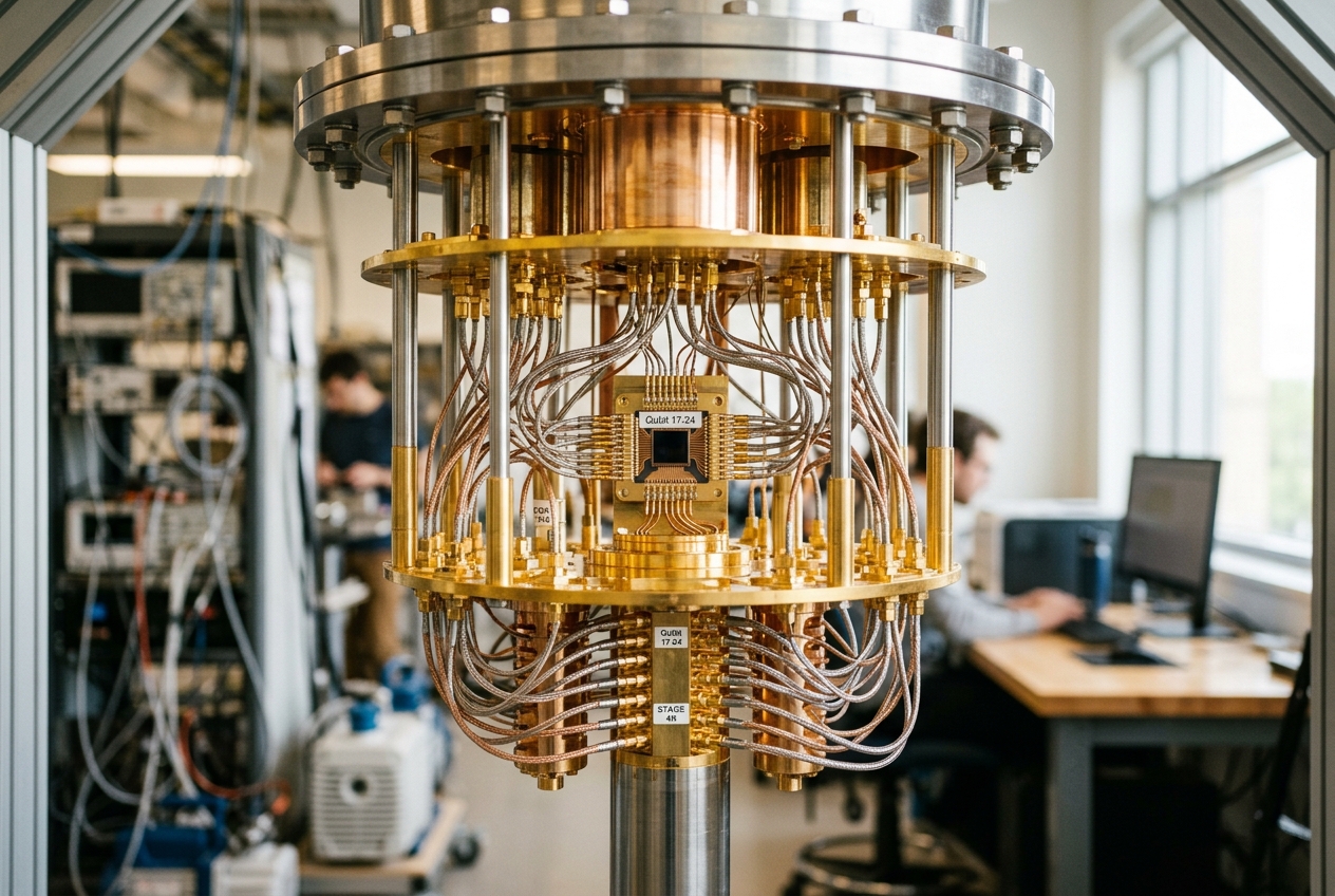
The leading physical implementation of quantum annealers uses superconducting circuits operating at millikelvin temperatures (typically $10\text{ mK}$ to $15\text{ mK}$, maintained via closed-cycle dilution refrigerators). The fundamental computational element is the rf-SQUID (Radio-Frequency Superconducting Quantum Interference Device) flux qubit.
An rf-SQUID consists of a continuous superconducting niobium or aluminum loop interrupted by one or more sub-micron Josephson tunnel junctions. When cooled below its critical superconducting transition temperature ($T_c \approx 9.2\text{ K}$ for Niobium), the loop exhibits zero electrical resistance, and magnetic flux through the loop is quantized in integer multiples of the magnetic flux quantum $\Phi_0 = \frac{h}{2e} \approx 2.067 \times 10^{-15}\text{ Wb}$.
- Circulating Currents as Pseudospins: When an external magnetic flux bias $\Phi_x^z \approx \frac{1}{2}\Phi_0$ is applied, the potential energy landscape forms a symmetric double-well potential. The two distinct minima correspond to macroscopic persistent currents circulating clockwise ($|R\rangle \equiv |\downarrow\rangle \equiv |1\rangle$) or counter-clockwise ($|L\rangle \equiv |\uparrow\rangle \equiv |0\rangle$).
- Tunable Transverse Driver: Applying an independent transverse flux bias $\Phi_x^x$ modifies the central barrier height between the two potential wells, controlling the quantum tunneling amplitude $\Delta(t)$ between $|L\rangle$ and $|R\rangle$, which corresponds to the transverse field coefficient $A(t) \sigma_i^x$.
- Inductive Couplers: Bilinear coupling between adjacent qubits is achieved through tunable mutual inductance loops ($M_{ij}$). By tuning the persistent current in an intermediary coupler rf-SQUID, the interaction strength $J_{ij} \sigma_i^z \sigma_j^z$ can be adjusted continuously from strong ferromagnetic ($J_{ij} < 0$) to strong anti-ferromagnetic ($J_{ij} > 0$) coupling.
Hardware Graph Topologies and Minor Embedding
Because superconducting planar fabrication is constrained to two dimensions, physical qubits cannot be wired with all-to-all connectivity. Commercial and research annealers rely on structured, sparse hardware interaction graphs:
- Chimera Topology: Arranged in unit cells of bipartite $K_{4,4}$ subgraphs with inter-cell connections, yielding an operational qubit degree of $d = 6$.
- Pegasus Topology: Introduces systematic coordinate offsets among diagonally interwoven qubit loops, expanding qubit connectivity to degree $d = 15$.
- Zephyr Topology: Utilizes a cross-clique geometric lattice providing node degrees of $d = 20$ or higher, reducing the overhead required to embed complex graphs.
Minor Embedding and Ferromagnetic Chains
Arbitrary real-world optimization problems typically present dense, non-planar interaction graphs $G_{\text{problem}} = (V_p, E_p)$ that do not natively match the physical hardware lattice $G_{\text{hardware}} = (V_h, E_h)$. To resolve this structural mismatch, compilers use minor embedding.
In minor embedding, a single logical variable $u \in V_p$ is mapped to a connected subtree (chain) of multiple physical qubits ${q_1, q_2, \dots, q_k} \subset V_h$. These physical qubits are tied together using strong ferromagnetic couplings:
$$J_{\text{chain}} \ll 0 \quad (|J_{\text{chain}}| \gg |h_i|, |J_{ij}|)$$
This penalty energetically favors identical spin alignments ($\sigma_{q_a}^z = \sigma_{q_b}^z$), forcing the entire chain to behave as a single effective logical spin.
However, minor embedding introduces three physical trade-offs: 1. Chain Breaks: If physical thermal noise or quantum fluctuations overcome $|J_{\text{chain}}|$, the chain fragments into contradictory states ($\sigma_{q_1}^z \neq \sigma_{q_k}^z$), introducing errors that require classical majority-voting heuristics to repair. 2. Qubit Overhead: Fully connecting a logical graph of $N$ variables on a hardware lattice with degree $d$ requires $O(N^2)$ physical qubits. 3. Dynamic Range Compression: Because hardware biases must remain within a finite physical range ($[-J_{\max}, +J_{\max}]$), setting a large $|J_{\text{chain}}|$ forces the problem couplings $J_{ij}$ to be rescaled to small values, making the computation more susceptible to analog noise.
Open-System Dynamics, Thermal Dissipation, and Analog Limitations
Unlike idealized mathematical formulations, commercial quantum annealers operate as open quantum systems interacting with a thermal bath:
$$\frac{d\rho}{dt} = -\frac{i}{\hbar}[H(t), \rho] + \mathcal{L}_{\text{diss}}(\rho)$$
where $\mathcal{L}_{\text{diss}}$ represents the Lindbladian dissipator capturing photon emission/absorption and environmental decoherence (detailed across Nature Physics and Physical Review Letters).
- Thermal Relaxation vs. Dephasing: While thermal dephasing destroys quantum phase coherence on nanosecond timescales, classical thermal relaxation can sometimes assist the computation: if the system is excited to a higher energy level during the sweep, interaction with the sub-Kelvin thermal bath can cool the system back into the ground state.
- Analog Control Precision and $J$-Chaos: Couplers and flux biases are programmed via digital-to-analog converters (DACs) subject to intrinsic $1/f$ magnetic flux noise and room-temperature quantization errors. If parameter misspecification perturbations ($\delta h_i, \delta J_{ij}$) exceed the energy gap between the ground state and low-lying excited states, the physical device solves a perturbed problem whose ground state differs from the target problem—a phenomenon known as $J$-chaos.
7. Comparative Analysis & Contemporary Landscape
Quantum Annealing is often evaluated alongside other prominent quantum paradigms, including universal Adiabatic Quantum Computation and gate-model architectures.
Stoquasticity and the Sign Problem
Current physical quantum annealers utilize stoquastic Hamiltonians—operators whose off-diagonal matrix elements in the computational basis are real and non-positive ($H_{ij} \le 0$ for $i \neq j$). Stoquastic Hamiltonians do not suffer from the infamous quantum Monte Carlo sign problem, meaning their equilibrium properties can often be efficiently simulated on classical high-performance computers using Path-Integral Quantum Monte Carlo (PIMC) or Spin-Vector Monte Carlo (SVMC).
Achieving universal Adiabatic Quantum Computation requires non-stoquastic Hamiltonians containing complex multi-body interactions (such as $\sigma_i^x \sigma_j^y$ or $\sigma_i^y \sigma_j^z$), which introduce destructive quantum interference that classical Monte Carlo methods cannot efficiently simulate.
Quantum Approximate Optimization Algorithm (QAOA)
On gate-model quantum processors (e.g., IBM Qiskit), optimization problems are approached through variational circuit algorithms like QAOA. QAOA acts as a Trotterized, discretized approximation of adiabatic evolution. The algorithm alternates between applying a problem unitary $U(C, \gamma) = e^{-i \gamma H_{\text{problem}}}$ and a driver mixer unitary $U(B, \beta) = e^{-i \beta H_{\text{init}}}$ across $p$ discrete layers:
$$|\gamma, \beta\rangle = \left( \prod_{k=1}^p e^{-i \beta_k H_{\text{init}}} e^{-i \gamma_k H_{\text{problem}}} \right) |+\rangle^{\otimes N}$$
While QAOA benefits from the precise error-mitigation and universal gate operations of circuit-based processors, current hardware implementations remain constrained to shallow circuit depths ($p \le 5$) and modest qubit counts due to gate infidelities and decoherence.
8. Real-World Applications Today
Major industrial and scientific organizations are actively benchmarking quantum annealing to tackle complex operational and scientific bottlenecks:
9. What This Means for You
It is easy to perceive quantum computing as a remote scientific curiosity confined to cryogenic research facilities. Yet the mathematical structures underlying quantum annealing directly intersect with the digital fabric of everyday life.
Consider modern personalized medicine. When a disease mutates, identifying a synthetic molecule capable of binding to the target pathogen requires calculating structural interaction energies across billions of possible molecular conformations.
Classical drug design relies on aggressive heuristic pruning that frequently discards promising therapeutic candidates because computing their interactions is too resource-intensive.
A mature quantum optimization framework can evaluate these complex combinatorial landscapes without resorting to arbitrary pruning. This shifts pharmaceutical discovery from brute-force trial-and-error toward direct, physics-based computation—shortening drug discovery timelines from years to days.
The same principles extend across critical civilian infrastructure. From stabilizing electrical distribution across renewable-dominated power grids to routing global supply chains during severe geopolitical disruptions, solving complex optimization problems more effectively creates tangible societal benefits: more reliable energy networks, reduced logistical overhead, and faster scientific discovery.
10. Today's Takeaway
Core Insight: Quantum annealing is an analog computing paradigm that reframes computational complexity as physical energy minimization: by transforming mathematical cost functions into superconducting Ising spin glasses and using quantum tunneling to traverse tall energy barriers, it provides an alternative path for navigating combinatorial problems that challenge classical computer architectures.
External References & Further Academic Study
- Lucas, A. (2014). Ising formulations of many NP problems. Frontiers in Physics / Andrew Lucas Formulation
- Johnson, M. W. et al. (2011). Quantum annealing with manufactured spins. Nature, 473(7346), 194–198
- Kadowaki, T., & Nishimori, H. (1998). Quantum annealing in the transverse Ising model. Physical Review E, 58(5), 5355
- Denchev, V. S. et al. (2016). What is the Computational Value of Finite-Range Tunneling? Physical Review X, 6(3), 031015
- Albash, T., & Lidar, D. A. (2018). Adiabatic quantum computation. Reviews of Modern Physics, 90(1), 015002