Eliassen-Palm (EP) Flux & Wave-Mean Flow Interaction: How Stratospheric Wave Drag and Transformed Eulerian Mean Dynamics Steer Planetary Zonal Jets

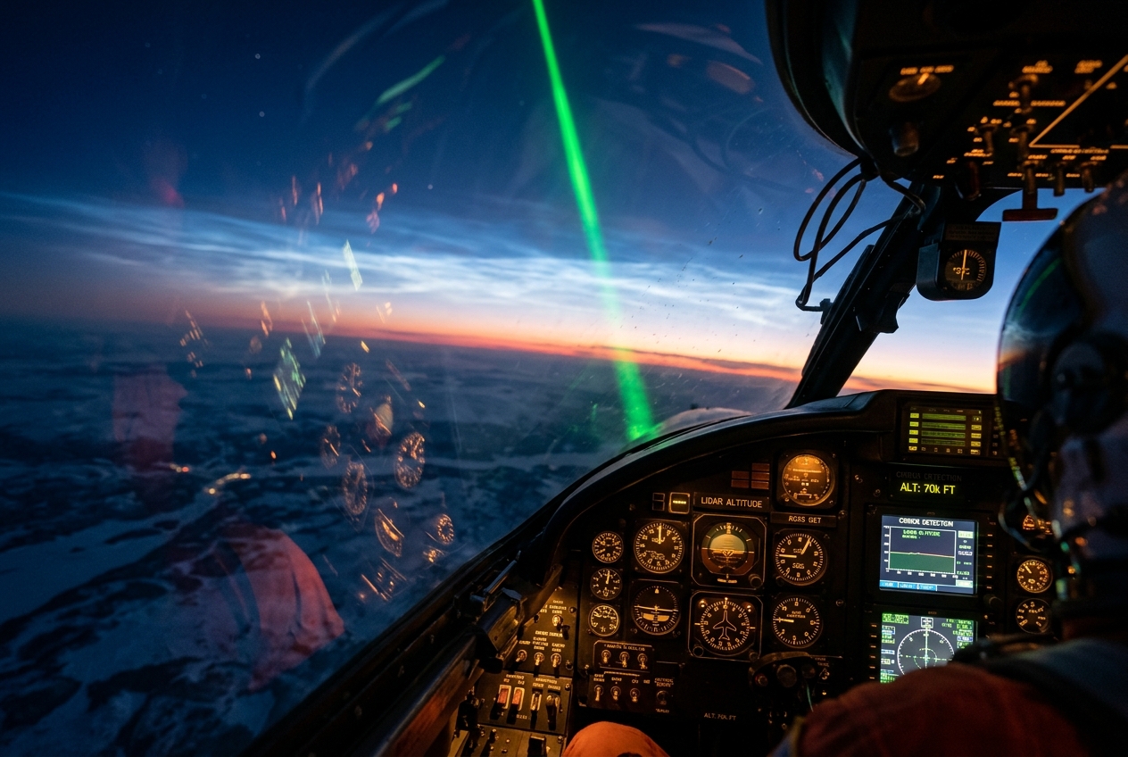
High above the snow-drifted spruce forests of northern Lapland, fifty miles north of the Arctic Circle, the midnight air at ground level is dead calm. The temperature hovers near $-32^\circ\text{C}$. The snow crystals on the ground squeak underfoot with the brittle, dry resonance peculiar to extreme sub-zero cold. If you look straight up into the pitch-black sky, past the pale green curtains of the aurora borealis, there is no visible sign of turbulence. The atmosphere feels immutable, frozen in place by the long polar night.

Yet twenty miles overhead, in the thin, ozone-rich air of the stratosphere, a planetary-scale catastrophe is unfolding.

For months, an immense vortex of hurricane-force winds has encircled the North Pole, spinning counterclockwise at speeds exceeding 180 miles per hour, acting as a deep atmospheric vault that locks the planet’s coldest air over the Arctic basin. But within the span of forty-eight hours, the barometer in your pocket begins a slow, mysterious descent. The high-altitude winds of the polar vortex are abruptly decelerating, coming to a dead halt, and violently reversing course to blow from the east. As the vortex disintegrates, the temperature in the middle stratosphere surges by an astonishing $40^\circ\text{C}$ in a matter of days—a phenomenon known as a sudden stratospheric warming.

               UPWARD WAVE PROPAGATION & VORTEX BREAKDOWN

      Stratosphere   [ Polar Vortex: u > 0 ]  <--- Wave Drag (\nabla·F < 0)
        (~30 km)                ^                       |
                                |  EP Flux Vector (F)   | Deceleration to
                                |  (Wave Energy &       | Easterlies (u < 0)
                                |   Momentum Flux)      v
      --------------------------|----------------------------------------
      Tropopause (~10 km)       |
                                |
      Troposphere    [ Planetary Rossby Waves ] ---> Surface Weather Extremes
        (Surface)    (Generated by Mountains &      (Cold Air Outbreaks)
                      Land-Sea Thermal Contrasts)

At the Earth's surface, you cannot see the giant waves crashing in the upper atmosphere. But within a fortnight, the broken pieces of that stratospheric engine will descend to the troposphere, altering the path of the North Atlantic jet stream and unlocking the Arctic vault to dump paralyzing blizzards and Siberian air across the mid-latitudes. What force could possibly reach thirty kilometers into the sky to shatter a vortex containing billions of tons of spinning air?

The answer lies in an invisible, elegant vector of wave-momentum transport known to dynamic meteorologists as the Eliassen–Palm (EP) flux.

2. What's Actually Happening: Plain English First

To understand how giant waves in the atmosphere can stop a jet stream in its tracks, we must first abandon the intuitive idea that waves merely transport water or air. In fluid dynamics, waves transport momentum and energy across immense distances without transporting the fluid itself.

Think of the Earth's atmosphere as a vast, rapidly rotating, layered fluid. In the lower atmosphere (the troposphere), wind blowing across massive north-south mountain ranges—such as the Rocky Mountains and the Tibetan Plateau—combined with sharp temperature contrasts between cold continents and warm oceans, forces giant ripples into the prevailing westerly winds. These planetary-scale undulations are called planetary waves or Rossby waves.

   POLE (Cold)
     ^      ___               ___               ___
     |     /   \             /   \             /   \      <-- Rossby Wave Crests
  y  |    /     \           /     \           /     \         (Warm Ridge)
     |   /       \         /       \         /       \
  0  +--/---------\-------/---------\-------/---------\---> x (Eastward)
     |             \     /           \     /           \
     |              \___/             \___/             \___/ <-- Rossby Wave Troughs
     v                                                        (Cold Trough)
   EQUATOR (Warm)

Imagine throwing a heavy stone into a tranquil pond. Ripples propagate outward in circles. As long as the ripples travel undisturbed through clean water, they carry energy silently. But when those ripples reach the shallow water near a sloping beach, they steepen, become unstable, and break. As they crash upon the sand, they deposit all their forward momentum onto the beach, pushing the sand and creating a longshore current.

In the atmosphere, planetary Rossby waves act exactly like those ocean swells. They are generated in the lower atmosphere, propagate vertically upward and equatorward into the stratosphere, and travel until they encounter a region where the background wind speeds match their own phase speed—a critical layer. Here, the waves can no longer propagate; they become non-linear, curl over, and "break" in the stratosphere.

When a wave breaks in the atmosphere, it deposits a powerful westward (retrograde) force onto the prevailing eastward (prograde) winds. If enough planetary waves surge upward and break simultaneously, this wave-induced drag can completely obliterate the circumpolar jet stream.

For decades, meteorologists struggled to calculate this drag correctly. When they looked at traditional weather charts and computed the classic average winds (the Eulerian mean), they observed a bizarre paradox: the eastward momentum pushed by swirling eddy winds seemed to be almost perfectly canceled out by the heat pushed by those same eddies. The atmosphere appeared to be full of fury, signifying nothing.

The breakthrough came when dynamicists realized that standard averages create mathematical optical illusions. To see the true, unvarnished force of atmospheric waves, one must combine eddy heat transport and eddy momentum transport into a single, unified vector: the Eliassen–Palm flux vector, $\mathbf{F}$. Wherever this vector converges ($\nabla \cdot \mathbf{F} < 0$), waves are breaking and acting as an absolute brake on the planetary circulation.

3. The Science: From Eulerian Fallacy to the Transformed Eulerian Mean (TEM)

3.1 The Eulerian Dilemma and the Charney–Drazin Non-Acceleration Theorem

To appreciate the necessity of the Eliassen–Palm flux, we must examine the classical Eulerian zonal-mean framework under Quasi-Geostrophic (QG) scaling on a mid-latitude $\beta$-plane. Let coordinates $(x, y, z)$ denote eastward, northward, and log-pressure height $z \equiv -H \ln(p / p_s)$, where $H \approx 7\,\text{km}$ is the atmospheric scale height, $p_s = 1000\,\text{hPa}$, and $\rho_0(z) = \rho_s e^{-z/H}$ is the basic-state density profile.

Decomposing any atmospheric field $\chi$ into a zonal mean $\overline{\chi}$ and an eddy perturbation $\chi'$: $$\chi(x, y, z, t) = \overline{\chi}(y, z, t) + \chi'(x, y, z, t), \quad \text{where } \overline{\chi} \equiv \frac{1}{2\pi a \cos\phi} \oint \chi \, dx$$

The standard Eulerian zonal-mean momentum and thermodynamic energy equations are:

$$\frac{\partial \overline{u}}{\partial t} - f_0 \overline{v} = -\frac{\partial (\overline{u'v'})}{\partial y} + \overline{X} \tag{1}$$

$$\frac{\partial \overline{\theta}}{\partial t} + \overline{w} \frac{\partial \theta_0}{\partial z} = -\frac{\partial (\overline{v'\theta'})}{\partial y} + \overline{Q} \tag{2}$$

where $f_0$ is the Coriolis parameter, $\theta_0(z)$ is the reference potential temperature, $\overline{u'v'}$ is the meridional eddy momentum flux, $\overline{v'\theta'}$ is the meridional eddy heat flux, $\overline{X}$ represents non-conservative friction, and $\overline{Q}$ represents diabatic heating.

Equation (1) suggests that the zonal wind $\overline{u}$ accelerates whenever there is a convergence of eddy momentum flux ($-\partial_y \overline{u'v'} > 0$). However, this is deeply misleading. In a baroclinic atmosphere, eddy heat flux convergence ($-\partial_y \overline{v'\theta'} \neq 0$) induces a secondary ageostrophic overturning circulation $(\overline{v}, \overline{w})$ via the mass continuity equation:

$$\frac{\partial \overline{v}}{\partial y} + \frac{1}{\rho_0} \frac{\partial (\rho_0 \overline{w})}{\partial z} = 0 \tag{3}$$

This secondary circulation produces a Coriolis torque $f_0 \overline{v}$ that acts in direct opposition to the eddy momentum flux convergence $-\partial_y \overline{u'v'}$.

In their landmark paper, Charney and Drazin (1961) proved the Non-Acceleration Theorem:

The Charney–Drazin Non-Acceleration Theorem: For small-amplitude, steady, unforced, adiabatic, and dissipationless planetary waves ($\overline{X} = 0, \overline{Q} = 0, \partial/\partial t = 0$), the Coriolis acceleration induced by the mean meridional circulation exactly balances the eddy momentum flux divergence: $$f_0 \overline{v} = \frac{\partial (\overline{u'v'})}{\partial y} \implies \frac{\partial \overline{u}}{\partial t} = 0$$

Under these ideal conditions, waves exert zero net acceleration on the mean zonal flow, despite the presence of vigorous, non-zero eddy heat and momentum fluxes. The classical Eulerian framework creates fictitious cancelation terms between the mean circulation and eddy fluxes, obscuring the true physical mechanism of wave-mean flow interaction.

3.2 The Transformed Eulerian Mean (TEM) Formulation

To eliminate these illusory compensation terms, Andrews and McIntyre (1976), building upon the foundational insights of Arnt Eliassen and Enok Palm (1961), introduced the Transformed Eulerian Mean (TEM) framework.

The TEM formulation defines a residual mean meridional circulation $(\overline{v}^, \overline{w}^)$ that subtracts the eddy-induced Stokes drift from the traditional Eulerian mean circulation:

$$\overline{v}^* \equiv \overline{v} - \frac{1}{\rho_0} \frac{\partial}{\partial z} \left( \rho_0 \frac{\overline{v'\theta'}}{\partial \theta_0 / \partial z} \right) \tag{4}$$

$$\overline{w}^* \equiv \overline{w} + \frac{\partial}{\partial y} \left( \frac{\overline{v'\theta'}}{\partial \theta_0 / \partial z} \right) \tag{5}$$

By substituting equations (4) and (5) into the Eulerian momentum and thermodynamic equations (1) and (2), the thermodynamic equation simplifies to a pure balance between residual advection and diabatic heating:

$$\frac{\partial \overline{\theta}}{\partial t} + \overline{w}^* \frac{\partial \theta_0}{\partial z} = \overline{Q} - \frac{1}{\rho_0}\frac{\partial}{\partial z}\left(\rho_0 \frac{\partial\overline{\theta'}}{\partial t}\right) \approx \overline{Q} \tag{6}$$

Simultaneously, the zonal-mean momentum equation transforms into:

$$\frac{\partial \overline{u}}{\partial t} - f_0 \overline{v}^* = \frac{1}{\rho_0} \nabla \cdot \mathbf{F} + \overline{X} \tag{7}$$

where $\mathbf{F} \equiv (F_y, F_z)$ is the Eliassen–Palm (EP) Flux Vector, defined in quasi-geostrophic log-pressure coordinates as:

$$F_y \equiv -\rho_0 \overline{u'v'} \tag{8a}$$

$$F_z \equiv \rho_0 f_0 \frac{\overline{v'\theta'}}{\partial \theta_0 / \partial z} = \rho_0 f_0 \frac{R}{H N^2} \overline{v' T'} \tag{8b}$$

Here, $N^2 \equiv \frac{g}{\theta_0}\frac{d\theta_0}{dz}$ is the Brunt–Väisälä buoyancy frequency, $R$ is the gas constant for dry air ($287\,\text{J}\,\text{kg}^{-1}\,\text{K}^{-1}$), and $T'$ is the temperature perturbation.

The two-dimensional divergence of the EP flux vector is:

$$\nabla \cdot \mathbf{F} \equiv \frac{\partial F_y}{\partial y} + \frac{\partial F_z}{\partial z} = -\frac{\partial (\rho_0 \overline{u'v'})}{\partial y} + \frac{\partial}{\partial z}\left( \rho_0 f_0 \frac{\overline{v'\theta'}}{\partial \theta_0 / \partial z} \right) \tag{9}$$

================================================================================
                    THE FUNDAMENTAL DYNAMICAL INSIGHT
================================================================================
 The divergence of the Eliassen–Palm flux, (1 / \rho_0) \nabla · F, represents 
 the ENTIRE, UNAMBIGUOUS NET FORCING exerted by transient and stationary eddies 
 on the mean zonal flow.

• \nabla · F > 0 (Divergence): Waves accelerate the zonal jet (westerly push)
   • \nabla · F < 0 (Convergence): Waves decelerate the zonal jet (easterly drag)
   • \nabla · F = 0 : Waves propagate without exerting any net force on the mean flow
================================================================================

Under the conditions of the Charney–Drazin theorem (steady, adiabatic, unforced linear waves), $\nabla \cdot \mathbf{F} \equiv 0$ identically throughout the domain. The TEM formulation reveals that the net wave forcing is zero without invoking fictitious cancellations between eddy terms and secondary circulations.

3.3 The EP Flux in Spherical Primitive Equation Coordinates

For diagnostic analysis using global atmospheric reanalysis datasets such as ECMWF ERA5 or NOAA NCEP/NCAR, the quasi-geostrophic Cartesian formulation is generalized to spherical log-pressure coordinates $(\lambda, \phi, z)$, where $\phi$ is latitude, $a$ is the Earth's mean radius ($6.371 \times 10^6\,\text{m}$), and $f = 2\Omega \sin\phi$:

$$F_\phi = \rho_0 a \cos\phi \left( \frac{\partial \overline{u}}{\partial z} \frac{\overline{v'\theta'}}{\partial \overline{\theta}/\partial z} - \overline{u'v'} \right) \tag{10a}$$

$$F_z = \rho_0 a \cos\phi \left( \left[ f - \frac{1}{a\cos\phi}\frac{\partial (\overline{u}\cos\phi)}{\partial \phi} \right] \frac{\overline{v'\theta'}}{\partial \overline{\theta}/\partial z} - \overline{u'w'} \right) \tag{10b}$$

Under quasi-geostrophic scaling on the sphere, equations (10a) and (10b) reduce to the standard diagnostic form:

$$F_\phi = -\rho_0 a \cos\phi \, \overline{u'v'} \tag{11a}$$

$$F_z = \rho_0 a \cos\phi \, f \frac{R}{H N^2} \overline{v' T'} \tag{11b}$$

The spherical divergence of the EP flux, representing the net zonal acceleration in units of $\text{m}\,\text{s}^{-2}$ (or $\text{m}\,\text{s}^{-1}\,\text{day}^{-1}$), is:

$$D_F \equiv \frac{1}{\rho_0 a \cos\phi} \nabla \cdot \mathbf{F} = \frac{1}{\rho_0 a \cos\phi} \left[ \frac{1}{a \cos\phi} \frac{\partial}{\partial \phi}(F_\phi \cos\phi) + \frac{\partial F_z}{\partial z} \right] \tag{12}$$

3.4 Physical Interpretation: Wave Action Flux and Group Velocity

The Eliassen–Palm flux vector has a profound physical meaning: it is proportional to the wave action flux vector.

For a packet of linear Rossby waves with local frequency $\omega$, zonal wavenumber $k$, and meridional wavenumber $l$, the wave action density $A$ is defined as the wave energy density $E$ divided by the intrinsic phase speed relative to the background flow $(c - \overline{u})$:

$$A \equiv \frac{E}{\omega - k\overline{u}} = -\frac{E}{k(\overline{u} - c)}$$

Andrews and McIntyre (1976) and Edmon et al. (1980) demonstrated that for conservative Rossby waves:

$$\mathbf{F} = \mathbf{c}_g A \tag{13}$$

where $\mathbf{c}g = (c{gy}, c_{gz})$ is the group velocity vector of the wave packet in the meridional plane.

                  EP FLUX CROSS-SECTION TRAJECTORIES

    Height (z)
      ^
 30 km|        \       |       /          <-- Wave Absorption / Convergence
      |         \      |      /               \nabla · F < 0 (Drag on Vortex)
      |          \     |     /
 20 km|           \    ^    /
      |            \   |   /              <-- Upward & Equatorward Propagation
      |             \  |  /                   F points parallel to group velocity c_g
 10 km|              \ | /
      |   ~~~~~~~~~~~~~V~~~~~~~~~~~~~~    <-- Tropopause Jet Core
  0 km+-----------------------------------> Latitude (\phi)
     Pole (90°N)    Midlat (45°N)   Equator (0°)

Because $\mathbf{F}$ points parallel to the group velocity vector $\mathbf{c}g$: 1. Arrows of $\mathbf{F}$ show the exact direction of wave energy propagation through the atmosphere. 2. In the troposphere, Rossby waves propagate upward ($F_z > 0$, driven by poleward heat flux $\overline{v'T'} > 0$) and equatorward ($F\phi < 0$, driven by poleward momentum flux $\overline{u'v'} > 0$). 3. Regions where EP flux arrows converge ($\nabla \cdot \mathbf{F} < 0$) mark locations where wave packets are breaking, losing their wave action density, and depositing westward momentum directly into the mean zonal flow.

3.5 Real-World Atmospheric Applications

Application A: Major Sudden Stratospheric Warmings (SSWs)

During boreal winter, planetary wave-1 and wave-2 structures propagate from the troposphere into the polar stratosphere. As these waves encounter their critical line near the polar night jet, $F_z$ increases dramatically, followed by extreme EP flux convergence: $$\frac{1}{\rho_0 a \cos\phi}\nabla \cdot \mathbf{F} \approx -20 \text{ to } -50\,\text{m}\,\text{s}^{-1}\,\text{day}^{-1}$$ This massive wave drag reverses the circumpolar westerlies ($\overline{u} > 0$) to easterlies ($\overline{u} < 0$). By equation (7), the strong wave drag drives a poleward residual circulation ($\overline{v}^ > 0$), which forces strong downward motion over the pole ($\overline{w}^ < 0$). Through equation (6), this downward motion causes intense adiabatic compression, warming the polar stratosphere by tens of degrees Celsius within days.

Application B: The Quasi-Biennial Oscillation (QBO)

In the equatorial stratosphere, the Quasi-Biennial Oscillation (a ~28-month downward-propagating cycle of alternating easterly and westerly zonal winds) is driven entirely by the vertical divergence of the EP flux. Upward-propagating equatorial Kelvin waves carry eastward momentum ($F_z > 0$, $\overline{u'w'} > 0$), dissipating to accelerate the westerly phase, while equatorial Rossby-gravity waves carry westward momentum ($F_z < 0$, $\overline{u'w'} < 0$), dissipating to accelerate the easterly phase.

3.6 Worked Analytical Example: Calculating Stratospheric Wave Drag

Let us perform a complete, realistic calculation of the EP flux divergence and the resulting zonal wind deceleration during an active planetary wave event in the sub-polar winter stratosphere.

Given Environmental Parameters:

• Latitude: $\phi = 60^\circ\text{N} \implies \cos(60^\circ) = 0.5, \quad \sin(60^\circ) = 0.866$
• Coriolis Parameter: $f_0 = 2 \times (7.292 \times 10^{-5}) \times 0.866 = 1.263 \times 10^{-4}\,\text{s}^{-1}$
• Earth Radius: $a = 6.371 \times 10^6\,\text{m}$
• Log-pressure Height: $z = 30\,\text{km} = 30,000\,\text{m}$
• Scale Height: $H = 7,000\,\text{m}$
• Air Density at $30\,\text{km}$: $\rho_0(z) = \rho_s e^{-z/H} = 1.225 \times e^{-30/7} = 1.225 \times 0.01376 = 0.01685\,\text{kg}\,\text{m}^{-3}$
• Buoyancy Frequency squared: $N^2 = 4.0 \times 10^{-4}\,\text{s}^{-2}$
• Gas Constant: $R = 287\,\text{J}\,\text{kg}^{-1}\,\text{K}^{-1}$

Observed Eddy Flux Gradients:

• Poleward Eddy Momentum Flux: $\overline{u'v'} = +15.0\,\text{m}^2\,\text{s}^{-2}$, with a meridional gradient over $\Delta y = 10^\circ \text{ latitude} \approx 1.11 \times 10^6\,\text{m}$ of $\frac{\partial \overline{u'v'}}{\partial y} = +1.2 \times 10^{-5}\,\text{m}\,\text{s}^{-2}$.
• Poleward Eddy Heat Flux: $\overline{v'T'} = +25.0\,\text{K}\,\text{m}\,\text{s}^{-1}$ at $z = 28\,\text{km}$, decreasing to $+5.0\,\text{K}\,\text{m}\,\text{s}^{-1}$ at $z = 32\,\text{km}$ due to severe wave breaking. Thus, over $\Delta z = 4,000\,\text{m}$: $$\frac{\partial \overline{v'T'}}{\partial z} = \frac{5.0 - 25.0}{4000} = -5.0 \times 10^{-3}\,\text{K}\,\text{s}^{-1}$$

Step 1: Compute the Horizontal Component $F_y$ and its Divergence

From equation (8a): $$F_y = -\rho_0 \overline{u'v'} = -(0.01685\,\text{kg}\,\text{m}^{-3}) \times (15.0\,\text{m}^2\,\text{s}^{-2}) = -0.2528\,\text{N}\,\text{m}^{-2}$$

The horizontal divergence term is: $$\frac{\partial F_y}{\partial y} = -\rho_0 \frac{\partial \overline{u'v'}}{\partial y} = -(0.01685) \times (1.2 \times 10^{-5}) = -2.022 \times 10^{-7}\,\text{N}\,\text{m}^{-3}$$

Step 2: Compute the Vertical Component $F_z$ and its Divergence

From equation (8b): $$F_z = \rho_0 f_0 \frac{R}{H N^2} \overline{v'T'}$$ Calculate the constant prefactor: $$\Gamma \equiv f_0 \frac{R}{H N^2} = \frac{(1.263 \times 10^{-4}\,\text{s}^{-1}) \times (287\,\text{J}\,\text{kg}^{-1}\,\text{K}^{-1})}{(7000\,\text{m}) \times (4.0 \times 10^{-4}\,\text{s}^{-2})} = \frac{0.03625}{2.80} = 0.01295\,\text{m}^{-1}$$

At $z = 30\,\text{km}$ (midpoint where $\overline{v'T'} = 15.0\,\text{K}\,\text{m}\,\text{s}^{-1}$): $$F_z = (0.01685\,\text{kg}\,\text{m}^{-3}) \times (0.01295\,\text{m}^{-1}) \times (15.0\,\text{K}\,\text{m}\,\text{s}^{-1}) = 3.273 \times 10^{-3}\,\text{N}\,\text{m}^{-2}$$

Now compute the vertical derivative $\frac{\partial F_z}{\partial z}$: $$\frac{\partial F_z}{\partial z} = \Gamma \frac{\partial (\rho_0 \overline{v'T'})}{\partial z} = \Gamma \left[ \rho_0 \frac{\partial \overline{v'T'}}{\partial z} + \overline{v'T'}\frac{d\rho_0}{dz} \right]$$ Since $\frac{d\rho_0}{dz} = -\frac{\rho_0}{H}$: $$\frac{\partial F_z}{\partial z} = \Gamma \rho_0 \left[ \frac{\partial \overline{v'T'}}{\partial z} - \frac{\overline{v'T'}}{H} \right]$$ Substitute our numerical values: $$\frac{\partial F_z}{\partial z} = (0.01295) \times (0.01685) \left[ -5.0 \times 10^{-3} - \frac{15.0}{7000} \right]$$ $$\frac{\partial F_z}{\partial z} = (2.182 \times 10^{-4}) \times \left[ -0.0050 - 0.002143 \right] = (2.182 \times 10^{-4}) \times (-0.007143) = -1.559 \times 10^{-6}\,\text{N}\,\text{m}^{-3}$$

Step 3: Total EP Flux Divergence and Net Flow Deceleration

Summing the horizontal and vertical contributions to obtain total divergence: $$\nabla \cdot \mathbf{F} = \frac{\partial F_y}{\partial y} + \frac{\partial F_z}{\partial z} = (-2.022 \times 10^{-7}) + (-1.559 \times 10^{-6}) = -1.761 \times 10^{-6}\,\text{N}\,\text{m}^{-3}$$

The net acceleration on the zonal-mean wind $\overline{u}$ is: $$\frac{\partial \overline{u}}{\partial t} = \frac{1}{\rho_0} \nabla \cdot \mathbf{F} = \frac{-1.761 \times 10^{-6}\,\text{N}\,\text{m}^{-3}}{0.01685\,\text{kg}\,\text{m}^{-3}} = -1.045 \times 10^{-4}\,\text{m}\,\text{s}^{-2}$$

Converting this acceleration into practical meteorological units ($\text{m}\,\text{s}^{-1}\,\text{day}^{-1}$): $$\frac{\partial \overline{u}}{\partial t} = (-1.045 \times 10^{-4}\,\text{m}\,\text{s}^{-2}) \times (86,400\,\text{s}\,\text{day}^{-1}) = \mathbf{-9.03\,\text{m}\,\text{s}^{-1}\,\text{day}^{-1}}$$

================================================================================
                        PHYSICAL INTERPRETATION OF RESULT
================================================================================
 In this region of the stratosphere, wave breaking generates an intense EP flux 
 convergence that decelerates the westerly polar vortex by approximately 
 9.0 meters per second EVERY SINGLE DAY.

Within just five to six days of sustained wave forcing of this magnitude, a 
 50 m/s westerly jet will be completely halted and forced into reverse, triggering 
 an official Major Sudden Stratospheric Warming.
================================================================================

3.7 Diagnostic Python Implementation (xarray, MetPy & NumPy)

Below is a complete, production-grade Python script designed to ingest atmospheric reanalysis data on pressure levels (such as from the ECMWF Open Data or Copernicus Climate Data Store), compute the spherical quasi-geostrophic Eliassen–Palm flux vector components $(F_\phi, F_z)$, evaluate their divergence, and generate a publication-ready latitude-height cross-section.

"""
================================================================================
Eliassen-Palm (EP) Flux Diagnostic Engine
Calculates QG EP Flux Vectors (F_phi, F_z) and EP Divergence in Log-p Coordinates
================================================================================
"""

import numpy as np
import xarray as xr
import matplotlib.pyplot as plt

def compute_ep_flux_cross_section(ds: xr.Dataset) -> xr.Dataset:
    """
    Computes the Eliassen-Palm Flux vector and its divergence from 3D gridded fields.

    Parameters:
    -----------
    ds : xr.Dataset containing:
        - u: Zonal wind (m/s), dimensions (time, level, lat, lon)
        - v: Meridional wind (m/s), dimensions (time, level, lat, lon)
        - T: Temperature (K), dimensions (time, level, lat, lon)
        - level: Pressure levels (hPa or Pa)
        - lat: Latitude in degrees (-90 to 90)
        - lon: Longitude in degrees (0 to 360)

    Returns:
    --------
    xr.Dataset with F_phi, F_z, and EP_div (m/s/day) on (level, lat).
    """
    # 1. Physical Constants
    a = 6.371e6          # Earth radius (m)
    omega = 7.292e-5      # Earth angular velocity (rad/s)
    g = 9.80665          # Gravitational acceleration (m/s^2)
    R = 287.05           # Dry air gas constant (J/kg/K)
    cp = 1004.0          # Specific heat at constant pressure (J/kg/K)
    kappa = R / cp       # 0.286
    p0 = 100000.0        # Reference surface pressure (Pa)
    H = 7000.0           # Atmospheric scale height (m)

# 2. Coordinate Extraction and Unit Standardization
    # Ensure pressure is in Pascals
    if ds['level'].max() < 2000.0:
        p = ds['level'] * 100.0
    else:
        p = ds['level']
    p = p.assign_attrs(units='Pa')

lat = ds['lat']
    phi = np.deg2rad(lat)
    cos_phi = np.cos(phi)
    sin_phi = np.sin(phi)
    f = 2.0 * omega * sin_phi  # Coriolis parameter (s^-1)

# Log-pressure height: z = -H * ln(p / p0)
    z = -H * np.log(p / p0)
    rho0 = (p0 / (R * 273.15)) * np.exp(-z / H)  # Basic state density profile

# 3. Zonal Averaging and Eddy Perturbations
    u = ds['u']
    v = ds['v']
    T = ds['T']

# Potential Temperature: theta = T * (p0 / p)^kappa
    theta = T * (p0 / p)**kappa

# Zonal means (denoted by bar)
    u_bar = u.mean(dim='lon')
    v_bar = v.mean(dim='lon')
    theta_bar = theta.mean(dim='lon')
    T_bar = T.mean(dim='lon')

# Perturbations (denoted by prime)
    u_prime = u - u_bar
    v_prime = v - v_bar
    theta_prime = theta - theta_bar
    T_prime = T - T_bar

# 4. Eddy Flux Covariances
    u_prime_v_prime = (u_prime * v_prime).mean(dim='lon')
    v_prime_theta_prime = (v_prime * theta_prime).mean(dim='lon')
    v_prime_T_prime = (v_prime * T_prime).mean(dim='lon')

# 5. Static Stability Parameter (N^2 in log-p coordinates)
    # d(theta_bar)/dz = -(p / H) * d(theta_bar)/dp
    dtheta_dp = theta_bar.differentiate(coord='level')
    dtheta_dz = -(p / H) * dtheta_dp

    # Buoyancy frequency squared N^2 = (g / theta_bar) * d(theta_bar)/dz
    N2 = (g / theta_bar) * dtheta_dz
    # Mask unphysically small or negative stability values
    N2 = xr.where(N2 < 1.0e-5, 1.0e-5, N2)

# 6. Compute EP Flux Components (Spherical QG Formulation)
    # F_phi = - rho0 * a * cos(phi) * [u'v']
    # F_z   =   rho0 * a * cos(phi) * f * (R / (H * N^2)) * [v'T']

    # Broadcasting coordinates across dimensions
    cos_phi_2d = cos_phi.broadcast_like(u_bar)
    f_2d = f.broadcast_like(u_bar)
    rho0_2d = rho0.broadcast_like(u_bar)

F_phi = -rho0_2d * a * cos_phi_2d * u_prime_v_prime
    F_z = rho0_2d * a * cos_phi_2d * f_2d * (R / (H * N2)) * v_prime_T_prime

# 7. Compute Spherical EP Flux Divergence
    # d/dphi (F_phi * cos_phi) / (a * cos_phi)
    F_phi_cos = F_phi * cos_phi_2d
    dF_phi_dphi = F_phi_cos.differentiate(coord='lat') * (180.0 / np.pi)  # rad derivative
    div_F_phi = (1.0 / (a * cos_phi_2d)) * dF_phi_dphi

# d(F_z)/dz = -(p / H) * d(F_z)/dp
    dF_z_dp = F_z.differentiate(coord='level')
    div_F_z = -(p / H) * dF_z_dp

# Net EP Divergence: (1 / (rho0 * a * cos_phi)) * \nabla \cdot F
    total_div_F = div_F_phi + div_F_z
    ep_acceleration = total_div_F / (rho0_2d * a * cos_phi_2d)  # m/s^2

# Convert to m/s/day
    ep_drag_per_day = ep_acceleration * 86400.0

# Package into resulting Dataset
    ep_ds = xr.Dataset(
        data_vars={
            'F_phi': F_phi.assign_attrs(units='kg/s^2', long_name='Meridional EP Flux'),
            'F_z': F_z.assign_attrs(units='kg/s^2', long_name='Vertical EP Flux'),
            'EP_div': ep_drag_per_day.assign_attrs(units='m/s/day', long_name='EP Flux Divergence'),
            'u_bar': u_bar.assign_attrs(units='m/s', long_name='Zonal Mean Zonal Wind')
        },
        coords={'level': ds['level'], 'lat': ds['lat']}
    )
    return ep_ds

def plot_ep_flux_diagnostic(ep_ds: xr.Dataset, title: str = "Eliassen-Palm Flux Diagnostic"):
    """
    Plots a cross-section of EP flux vectors over contours of EP divergence and zonal wind.
    """
    lat = ep_ds['lat']
    plev = ep_ds['level']
    u_mean = ep_ds['u_bar']
    ep_div = ep_ds['EP_div']

    # Scale EP vectors for visual clarity across pressure levels
    # F_phi and F_z have radically different numerical ranges
    F_phi_scaled = ep_ds['F_phi'] / np.maximum(np.abs(ep_ds['F_phi']).max(), 1e-5)
    F_z_scaled = (ep_ds['F_z'] / np.maximum(np.abs(ep_ds['F_z']).max(), 1e-5)) * 1.5

fig, ax = plt.subplots(figsize=(12, 7))

# 1. Shading: EP Flux Divergence (Wave Drag in m/s/day)
    div_levels = np.arange(-15, 16, 2.5)
    cf = ax.contourf(lat, plev, ep_div, levels=div_levels, cmap='RdBu_r', extend='both')
    cbar = plt.colorbar(cf, ax=ax, orientation='vertical', pad=0.02)
    cbar.set_label(r'$\frac{1}{\rho_0 a \cos\phi} \nabla \cdot \mathbf{F}$ (m s$^{-1}$ day$^{-1}$)', fontsize=12)

# 2. Contours: Zonal-Mean Zonal Wind (\bar{u})
    u_levels = np.arange(-30, 90, 10)
    cs = ax.contour(lat, plev, u_mean, levels=u_levels, colors='black', linewidths=1.2)
    ax.clabel(cs, inline=True, fontsize=9, fmt='%d m/s')

# 3. Quivers: Eliassen-Palm Flux Vectors
    # Subsample grid for legible quiver plotting
    skip_lat = slice(None, None, 4)
    skip_p = slice(None, None, 2)

    Q = ax.quiver(
        lat[skip_lat], plev[skip_p],
        F_phi_scaled.values[skip_p, skip_lat],
        -F_z_scaled.values[skip_p, skip_lat],  # Inverted because p-axis decreases upward
        color='gold', scale=25, width=0.0035, headwidth=4, headlength=5, edgecolors='k', linewidth=0.5
    )

ax.set_yscale('log')
    ax.invert_yaxis()
    ax.set_ylim([1000, 10])
    ax.set_xlim([0, 90])
    ax.set_xlabel('Latitude (°N)', fontsize=12)
    ax.set_ylabel('Pressure Level (hPa)', fontsize=12)
    ax.set_title(title, fontsize=14, fontweight='bold')
    ax.grid(True, linestyle='--', alpha=0.5)

plt.tight_layout()
    plt.show()

4. Practical Outdoor Guidance

While the Eliassen–Palm flux is computed in the rarefied heights of the stratosphere, its consequences govern the large-scale weather patterns experienced on the ground. A keen observer equipped with simple instruments can detect the surface footprint of these planetary wave-breaking events.

+--------------------------------------------------------------------------------+
|                   OBSERVATIONAL MANIFESTATIONS AT GROUND LEVEL                 |
+================================================================================+
| 1. Barometric Trends:                                                          |
|    When an intense upward EP flux pulse breaks in the stratosphere, the polar  |
|    vortex collapses, triggering a transition to a strongly negative Arctic     |
|    Oscillation (AO) / North Atlantic Oscillation (NAO). At mid-latitudes,      |
|    watch for a sustained barometric rise over Greenland and the Arctic         |
|    accompanied by a persistent pressure drop over the Azores and Western       |
|    Europe.                                                                     |
|                                                                                |
| 2. Cloud Signatures & Jet Stream Buckling:                                     |
|    Observe high-altitude cirrus filaments (*cirrus uncinus* or "mare's tails"). |
|    When planetary waves are actively breaking, the jet stream buckles into     |
|    extreme meridional excursions. High clouds will no longer stream purely     |
|    west-to-east; they will surge from the deep south (warm ridge) or dive from |
|    the northwest (cold trough) at speeds exceeding 100 knots.                  |
|                                                                                |
| 3. Surface Wind Direction & Temperature Advection:                             |
|    Following stratospheric EP flux convergence by 10 to 14 days, the surface   |
|    storm track shifts equatorward. In Western Europe and North America, watch   |
|    for prevailing westerly winds to break down into persistent, frigid         |
|    northeasterly or easterly winds (the classic "Beast from the East" setup).  |
+--------------------------------------------------------------------------------+

The Outdoor Enthusiast's Rule of Thumb

• For the Hiker and Mountaineer: When winter weather apps show a "Polar Vortex Split" or "Sudden Stratospheric Warming", do not look for immediate storms the next morning. Mark your calendar two weeks forward. The downward propagation of wave-drag anomalies takes 10 to 18 days to reach the surface, after which prolonged, blocking high-pressure systems will lock freezing arctic air over mid-latitude mountain ranges for weeks at a time.
• For the Sailor: Watch the high-altitude pressure systems tracked by national agencies like the NOAA Climate Prediction Center and the UK Met Office. A sudden surge in vertical EP flux at $100\,\text{hPa}$ signals that the mid-latitude westerlies will soon weaken, leading to erratic, meandering storm tracks and sudden, un-forecast gale shifts in the open ocean.

5. Today's Meteorological Rule of Thumb

The Eliassen–Palm Imperative: Atmospheric waves do not push the wind where they travel; they push the wind where they die. Wherever the Eliassen–Palm flux arrows point, wave energy is flowing—but wherever those arrows crash together and terminate ($\nabla \cdot \mathbf{F} < 0$), the sky is slamming on the brakes, halting jet streams and reshaping the weather of the globe.

Authoritative Meteorological References & Further Reading

1. World Meteorological Organization (WMO) Scientific Assessment of Stratospheric Dynamics
2. ECMWF ERA5 Atmospheric Dynamics & Reanalysis Documentation
3. NOAA Climate Prediction Center: Stratosphere-Troposphere Monitoring Diagnostics
4. Met Office Hadley Centre: Sudden Stratospheric Warmings and Jet Stream Dynamics
5. American Meteorological Society (AMS) Glossary: Eliassen-Palm Flux Vector