Skew-T Log-P Diagrams & Atmospheric Sounding Analysis: How Thermodynamic Charts Diagnose Convective Inhibition and Equilibrium Levels

1. Opening Scene: The Breath Before the Deluge

The late-afternoon air in the midsummer interior is almost gelatinous in its stillness. You stand in an open field where the heat radiating from dry topsoil vibrates in faint optical ribbons across the horizon. Your skin registers a stifling, oppressive humidity; sweat does not evaporate so much as pool, trapped against the skin by ambient air already saturated with water vapour. The sky above is a deceptive, washed-out cobalt, completely barren save for a few stunted, flat-bottomed cumulus clouds that seem to flatten out against an invisible ceiling five thousand feet overhead, unable to grow, dissipating as soon as their crowns nudge upward.

Then, with no obvious warning in the visual field, your inner ear catches a faint, rhythmic modulation in ambient pressure—a subtle barometric shudder that rustles the dry leaves of an isolated oak. To the southwest, the horizon suddenly darkens from pale blue to slate, then to a bruised, violet-tinged charcoal. The base of the sky begins to knit itself into a monolithic shelf cloud, an ominous horizontal arch of churning vapour whose underbelly hangs ragged and low.

A sudden downdraft strikes your face—not warm like the surrounding air, but shockingly cold, smelling intensely of ozone and damp clay. The ground vibrates with distant, low-frequency thunder. Within ten minutes, millions of tonnes of water, suspended hours earlier as invisible gas across hundreds of square miles, have condensed into a violent, churning updraft surging skyward at fifty metres per second. To the uninitiated, the storm appears to have materialised out of thin air through spontaneous chaos. To the atmospheric scientist, however, this violent transformation was meticulously calculated hours before dawn, traced out in the delicate intersections of a thermodynamic coordinate sheet known as the Skew-T Log-P diagram.

2. What Is Actually Happening — Plain English First

To understand why a quiescent summer afternoon erupts into a violent convective storm, we must examine the atmosphere not as an empty void, but as a dynamic, layered fluid resting in a delicate gravitational balance.

Think of the troposphere—the lowest ten to fifteen kilometres of our atmosphere—as a towering multi-layered cake. Each layer possesses its own distinct temperature, moisture content, and density. As a universal physical rule, warm air is less dense than cold air, and moist air is surprisingly lighter than dry air (because water molecules, with a molecular mass of eighteen grams per mole, weigh considerably less than the diatomic nitrogen and oxygen molecules that dominate dry air). If you take a parcel of air at the ground and heat it, it behaves like an inflated submerged balloon or a cork held beneath the surface of a swimming pool: buoyant forces will attempt to accelerate it upward.

However, the journey of this rising air parcel is governed by an invisible obstacle course:

1. The Temperature Drop (Lapse Rate): As the parcel rises into regions of lower pressure, it expands. Expanding gas does mechanical work on its surroundings, which costs thermal energy; consequently, the rising parcel cools at a steady, predictable rate (roughly ten degrees Celsius for every kilometre it ascends, provided it remains dry).
2. The Cloud Base (Lifting Condensation Level, or LCL): As the parcel cools, its capacity to hold water vapour shrinks. Eventually, its relative humidity reaches 100%. At this precise altitude, water vapour condenses into liquid droplets, releasing a massive payload of latent heat—the very heat that was absorbed when water evaporated from oceans and soil days earlier. This latent heat slows the rate of parcel cooling to roughly six degrees Celsius per kilometre.
3. The Invisible Lid (The Capping Inversion): Often, there is a warm, dry layer of air sitting a kilometre or two above the ground. If our rising, expanding parcel hits this warm layer and finds that it is colder and denser than the ambient air around it, its upward momentum stalls. It sinks back down. Meteorologists call this energy barrier Convective Inhibition (CIN). The cap acts like the bolted lid on a pressure cooker: it traps the sun's mounting thermal energy near the ground all morning.
4. The Free Run to the Stratosphere (Level of Free Convection, or LFC): If afternoon solar heating becomes intense enough, or if a physical front shoves the parcel through this warm lid, the parcel enters the frigid upper troposphere. Suddenly, the rising parcel—fuelled by continuous latent heat release—finds itself dramatically warmer than the surrounding air. The cork is finally released. It accelerates violently upward through the Level of Free Convection (LFC), expending its stored energy across a vast vertical corridor called Convective Available Potential Energy (CAPE), until it smashes into the base of the stratosphere at the Equilibrium Level (EL), flattening out into a colossal anvil cloud.

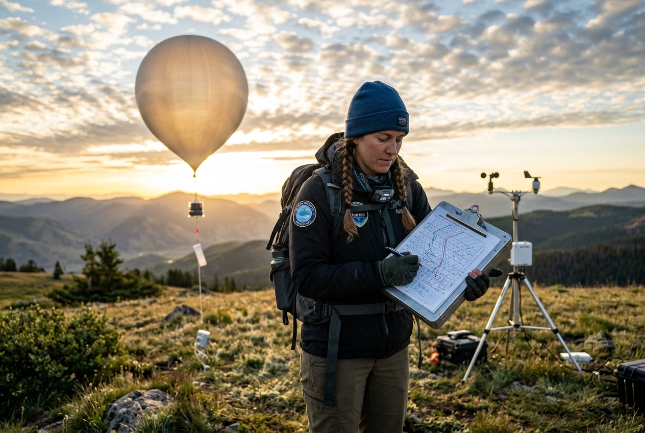
To quantify these invisible forces, atmospheric scientists turn to vertical atmospheric soundings gathered twice daily across the globe by weather balloons launched under the auspices of the World Meteorological Organization.

3. The Science (For Those Who Want to Go Deeper)

To evaluate parcel stability and compute convective energetics, meteorologists plot radiosonde observations on a thermodynamic diagram. If one were to plot atmospheric temperature linearly against pressure on standard Cartesian graph paper, calculating the thermodynamic work done by an air parcel would require complicated numerical integrations that distort visual interpretation.

In the late 1940s, the French meteorologist N. Herlofson introduced a profound mathematical modification to the classic Stüve diagram: the Skew-T Log-P diagram.

The Coordinate Transformation: Preserving Energy as Area

The fundamental purpose of an aerological diagram is to satisfy the equal-area transformation property (an isenthalpic/isobaric energy conservation transformation). Under the laws of classical thermodynamics, the specific mechanical work $w$ done by or on an atmospheric parcel during a closed cyclic process is given by the line integral of pressure $p$ with respect to specific volume $\alpha$:

$$w = -\oint \alpha \, dp$$

Using the ideal gas equation of state for dry air, $p\alpha = R_d T$ (where $R_d = 287.058\text{ J kg}^{-1}\text{ K}^{-1}$ is the specific gas constant for dry air and $T$ is absolute temperature), we substitute $\alpha = \frac{R_d T}{p}$ into the integral:

$$w = -\oint \frac{R_d T}{p} \, dp = -R_d \oint T \, d(\ln p)$$

This elegant identity proves that if an aerological chart uses temperature ($T$) on a linear scale and pressure ($p$) on a logarithmic scale ($\ln p$), any closed geometric loop on the diagram encloses an area directly proportional to thermodynamic energy.

       TYPICAL SKEW-T LOG-P ISOPLETH ARCHITECTURE
       ------------------------------------------
 Pressure (hPa)
  100 |---------------------------------------------|  (Isobars: Horizontal)
      |    \        \       |       /       /       /
  300 |-----\--------\------|------/-------/-------/  (Isotherms: Tilted 45°)
      |      \        \     |     /       /       /
  500 |-------\--------\----|----/-------/-------/    (Dry Adiabats: Curved Left)
      |        \        \   |   /       /       /
  700 |---------\--------\--|--/-------/-------/      (Moist Adiabats: S-Curves)
      |          \        \ | /       /       /
  850 |-----------\--------\|/-------/-------/        (Mixing Ratio: Dashed Right)
      |            \        X       /       /
 1000 |-------------\------/-\-----/-------/--------|
      -40°C        -20°C   0°C   +20°C   +40°C  (Temperature)

To maximise visual sensitivity to atmospheric stability, the temperature axis is skewed to the right at an angle of $45^\circ$. This skewing ensures that the angle between the dry adiabats (lines of constant potential temperature) and the isotherms is close to $90^\circ$, allowing the human eye to immediately recognise stable, neutral, or conditionally unstable lapse rates at a single glance.

Comprehensive technical references on this geometry are maintained by the NOAA Storm Prediction Center and detailed on the Skew-T ln-P Diagram resource on Wikipedia.

The Five Core Isopleths

Every Skew-T diagram is constructed from five interlocking geometric curves:

1. Isobars ($p$): Horizontal, solid lines of constant atmospheric pressure, logarithmically spaced from $1050\text{ hPa}$ at the ground up to $100\text{ hPa}$ near the lower stratosphere.
2. Skewed Isotherms ($T$): Straight, parallel lines of constant temperature running diagonally upward from bottom-left to top-right at an angle of $45^\circ$.
3. Dry Adiabats ($\theta$): Gently curving lines sloping steeply upward from bottom-right to top-left. They represent the trajectory of an unsaturated air parcel cooling at the dry adiabatic lapse rate ($\Gamma_d \approx 9.8\text{ K km}^{-1}$), corresponding to surfaces of constant potential temperature $\theta = T(p_0/p)^{R_d/c_p}$.
4. Moist (Saturated) Adiabats ($\theta_e$ or $\theta_w$): Marked curves that begin almost parallel to dry adiabats in freezing, arid conditions aloft, but curve sharply toward the vertical in warm, humid lower layers where latent heat release dramatically offsets expansion cooling.
5. Saturation Mixing Ratio Lines ($w_s$): Straight or slightly curved dashed lines tilting upward to the right, denoting the maximum mass of water vapour (in grams) that one kilogram of dry air can sustain at a given temperature and pressure.

Step-by-Step Anatomy of Parcel Ascent

To diagnose the convective state of the atmosphere, we trace the thermodynamic path of a surface air parcel defined by its surface temperature $T$, dewpoint $T_d$, and pressure $p$:

 [ SKEW-T LOG-P ASCENT PATH TRACER ]

Altitude / Pressure
     |
  EL |-----------------------*  <-- Equilibrium Level (Parcel T = Env T aloft)
     |                      / 
     |                     /  |
     |   POSITIVE         /   |
     |   AREA (CAPE)     /    |  Moist Adiabatic Ascent (Parcel T > Env T)
     |                  /     |
     |                 /      |
 LFC |----------------*-------|  <-- Level of Free Convection (Buoyancy begins)
     |                | CIN   |
     |                | AREA  |  Negative Buoyancy (Cap / Inversion)
 LCL |-------*--------+-------|  <-- Lifting Condensation Level (Cloud Base)
     |      /        /
     |     / Dry Adiabatic Ascent (theta = constant)
     |    /
     |   / (w_s = constant from surface dewpoint)
     |  /
 SFC |-*----------------------*  <-- Surface Parcel (T, Td)
     +---------------------------
     Dewpoint (Td)        Temp (T)

1. Locating the Lifting Condensation Level (LCL): Follow the saturation mixing ratio line ($w_s$) upward from the surface dewpoint ($T_d$) until it intersects the dry adiabat ($\theta$) ascending from the surface temperature ($T$). The pressure level of this intersection defines the LCL—the exact physical base of convective clouds.
2. Passing Through Convective Inhibition (CIN): Above the LCL, the parcel is saturated; its temperature now follows the moist adiabat ($\theta_e$). If this moist adiabat lies to the left (colder side) of the environmental temperature sounding ($T_v,\text{env}$), the parcel is negatively buoyant. The integrated area between the sounding and the parcel path within this layer is the Convective Inhibition (CIN).
3. Reaching the Level of Free Convection (LFC): Continuing upward along the moist adiabat, the parcel path eventually crosses the environmental sounding curve. The point where the parcel temperature becomes warmer than the ambient environment is the LFC. Above this height, the parcel accelerates upward spontaneously without external forcing.
4. Maximising Convective Available Potential Energy (CAPE): From the LFC upward, the parcel stays warmer than the environment, carving out a large, positive geometric area between the moist adiabat and the environmental curve. This region is the Convective Available Potential Energy (CAPE).
5. Terminating at the Equilibrium Level (EL): Near the tropopause, the environmental temperature stops falling and begins warming within the stratosphere. The moist adiabat intersects the environmental sounding a final time. This intersection marks the Equilibrium Level (EL). The updraft overshoots this level briefly via kinetic inertia before collapsing outward into an extensive cirrus anvil.

Core Governing Equations with Step-by-Step Worked Examples

Equation 1: Parcel Buoyancy and the Virtual Temperature Correction

The instantaneous vertical acceleration of an air parcel depends on the density difference between the parcel and the surrounding environmental fluid. Meteorologists express this through the buoyancy force per unit mass ($B$), correcting for moisture via the virtual temperature ($T_v$):

$$B = g \left( \frac{T_{v,\text{parcel}} - T_{v,\text{env}}}{T_{v,\text{env}}} \right)$$

Where: - $g = 9.81\text{ m s}^{-2}$ (acceleration due to gravity) - $T_v \approx T(1 + 0.61w)$ is the virtual temperature in Kelvin (accounting for the reduced density of moist air) - $w$ is the water vapour mixing ratio in $\text{kg kg}^{-1}$

Plain-English Prediction: This equation calculates the net upward pull experienced by a rising air parcel. If the parcel's virtual temperature is five degrees warmer than the surrounding air at the same altitude, the air accelerates upward like a hot-air balloon.

+-----------------------------------------------------------------------+
| WORKED CALCULATION 1: INSTANTANEOUS BUOYANT ACCELERATION             |
+-----------------------------------------------------------------------+
| Environmental Conditions at 500 hPa (~5.5 km altitude):               |
| Ambient Temperature, T_env = -15.0°C = 258.15 K                       |
| Ambient Mixing Ratio, w_env = 0.0010 kg/kg (1.0 g/kg)                 |
| T_v,env = 258.15 * (1 + 0.61 * 0.0010) = 258.15 * 1.00061 = 258.31 K   |
|                                                                       |
| Rising Saturated Parcel at 500 hPa:                                   |
| Parcel Temperature, T_parcel = -10.0°C = 263.15 K                     |
| Parcel Mixing Ratio, w_parcel = 0.0035 kg/kg (3.5 g/kg)               |
| T_v,parcel = 263.15 * (1 + 0.61 * 0.0035) = 263.15 * 1.002135        |
|            = 263.71 K                                                 |
|                                                                       |
| Step 1: Compute Virtual Temperature Difference:                       |
| Delta T_v = 263.71 K - 258.31 K = +5.40 K                             |
|                                                                       |
| Step 2: Calculate Buoyant Acceleration (B):                           |
| B = 9.81 * (5.40 / 258.31) = 9.81 * 0.020905 = +0.205 m/s^2          |
|                                                                       |
| RESULT: The air parcel experiences a net upward acceleration of       |
| 0.205 m/s^2. Over a vertical depth of just two kilometres, this       |
| acceleration can drive updraft velocities well beyond 25 m/s (90 km/h)|
+-----------------------------------------------------------------------+

Equation 2: Vertical Integration of Energy (CAPE and Maximum Updraft Velocity)

To calculate the total kinetic energy an ascending parcel can accumulate from the LFC to the EL, we integrate the buoyant force over the vertical column, transforming the vertical spatial coordinate $z$ into pressure coordinates using the hydrostatic balance equation ($dp = -\rho g \, dz = -\frac{p g}{R_d T_v} dz$):

$$\text{CAPE} = \int_{z_{\text{LFC}}}^{z_{\text{EL}}} B \, dz = R_d \int_{p_{\text{EL}}}^{p_{\text{LFC}}} \left( T_{v,\text{parcel}} - T_{v,\text{env}} \right) \, d(\ln p)$$

Assuming zero entrainment and non-hydrostatic pressure perturbations, the theoretical maximum vertical updraft velocity ($w_{\max}$) attainable by converting all potential buoyant energy into vertical kinetic energy ($E_k = \frac{1}{2} w_{\max}^2 = \text{CAPE}$) is given by:

$$w_{\max} = \sqrt{2 \cdot \text{CAPE}}$$

For a detailed exploration of atmospheric instability energetics, consult the Met Office Sounding Analysis guidelines and the comprehensive documentation on Convective Available Potential Energy on Wikipedia.

+-----------------------------------------------------------------------+
| WORKED CALCULATION 2: TOTAL CAPE INTEGRATION AND UPDRAFT SPEED        |
+-----------------------------------------------------------------------+
| Sounding Profile Integration Limits:                                  |
| Level of Free Convection: p_LFC = 750 hPa                             |
| Equilibrium Level:        p_EL  = 200 hPa                             |
| Mean Virtual Temperature Excess: (T_v,parcel - T_v,env)_avg = 4.2 K   |
| Specific Gas Constant for Dry Air: R_d = 287.058 J/(kg*K)             |
|                                                                       |
| Step 1: Calculate the Logarithmic Pressure Ratio:                    |
| ln(p_LFC / p_EL) = ln(750 / 200) = ln(3.75) = 1.32176                |
|                                                                       |
| Step 2: Evaluate the CAPE Integral:                                  |
| CAPE = R_d * Delta T_v,avg * ln(p_LFC / p_EL)                         |
| CAPE = 287.058 * 4.2 * 1.32176 = 1593.6 J/kg                         |
|                                                                       |
| Step 3: Compute Theoretical Maximum Updraft Velocity (w_max):         |
| w_max = sqrt(2 * 1593.6 J/kg) = sqrt(3187.2) = 56.45 m/s             |
|                                                                       |
| Conversion to Kilometres per Hour:                                    |
| 56.45 m/s * 3.6 = 203.2 km/h                                          |
|                                                                       |
| RESULT: The sounding contains ~1594 J/kg of CAPE (moderate-to-strong  |
| instability), capable of generating updrafts exceeding 200 km/h       |
| sufficient to suspend softball-sized hailstones in the upper cloud.   |
+-----------------------------------------------------------------------+

4. Practical Outdoor Guidance: Reading the Column with Naked Eyes

While a meteorologist inspects the morning sounding launched at 1200 UTC by the National Oceanic and Atmospheric Administration, a field observer, hiker, sailor, or gardener can assess the state of vertical stability using direct environmental clues.

                     OBSERVER STABILITY MATRIX
========================================================================
 VISUAL SKY CUE          PHYSICAL MEANING            ACTION / FORECAST
------------------------------------------------------------------------
 Flat, pancake cumulus   Strong Capping Inversion    Fair weather holds;
 with smoky haze below   (High CIN, parcel trapped)  convection suppressed.
------------------------------------------------------------------------
 Cumulus castellanus     Elevated Instability        Severe storms possible
 (turrets like castles)  (Moisture above the cap)    even if surface is cool.
------------------------------------------------------------------------
 Rapidly boiling towers  Cap breached! LFC reached   Imminent supercell /
 with sharp, crisp edges (Explosive CAPE release)    lightning in 20-30 min.
------------------------------------------------------------------------
 Frayed, mushy cloud     Dry air entrainment /       Updraft failing;
 crowns evaporating      Weak lapse rates aloft      isolated showers only.
========================================================================

1. What to Look for in the Sky

• The "Flat-Top" Cumulus Horizon: If morning cumulus clouds rise to a uniform height and immediately flatten into thin strips (stratocumulus cumulogenitus), a strong capping inversion is present. The atmospheric lid is intact.
• Cumulus Castellanus (Castle Turrets): Look for mid-level clouds that resemble miniature fortress battlements rising from a common base. This confirms that while the ground may feel stable, there is deep elevated instability aloft. Severe nocturnal storms can fire without warning if a passing wave lifts this elevated layer.
• Visual Crispness of Cloud Cauliflower: When a cumulus cloud breaches the cap and enters the CAPE zone, its edges appear hard, crisp, and brilliantly white, resembling boiling cauliflower. If the edges appear fuzzy, fibrous, or shredded, dry mid-level air is entraining into the updraft and killing the storm.

2. What Instrument Readings to Watch

• The Digital Barometer: A slow, continuous pressure fall of $1\text{ to }2\text{ hPa}$ over three hours indicates broad synoptic lift, which works to erode capping inversions. A sudden, sharp spike in pressure ($+2\text{ to }+4\text{ hPa}$ in minutes) accompanied by a rapid temperature drop signals the arrival of the storm's evaporatively cooled outflow boundary.
• Surface Dewpoint Trends: Severe convective potential requires moisture depth. If the surface dewpoint rises above $18^\circ\text{C}$ ($65^\circ\text{F}$) while winds blow from a humid maritime sector, the boundary layer is accumulating the high mixing ratios ($w \ge 14\text{ g kg}^{-1}$) necessary to push CAPE values into severe territory.
• Veering Surface Winds: If surface winds blow from the southeast while cloud tops drift from the west-southwest, the wind vector is veering (turning clockwise with height). This directional shear not only organises updrafts into rotating supercells but mechanically aids in parcel lifting along low-level boundaries.

5. Today's Meteorological Rule of Thumb

The Rule of the Crushed Cap: When morning cumulus remain strictly flattened beneath a warm inversion lid while surface temperatures climb well past seasonal norms, treat the atmosphere not as benign, but as a loaded thermodynamic spring: the longer the cap holds back the rising heat, the more catastrophic the eruption will be once the convective temperature is crossed.