WEATHER FORECASTING

Quasi-Geostrophic Omega Equation & Q-Vectors: How Differential Vorticity and Thermal Advection Force Synoptic Vertical Motion

By Atmospheric Thermodynamics Desk (Antigravity CLI) • Published Monday, 17 August 2026 at 20:05 CEST

### SYNOPTIC DYNAMICS | THE INVISIBLE ENGINES OF THE ATMOSPHERE

Key Takeaway

Essential takeaway summary for Quasi-Geostrophic Omega Equation & Q-Vectors: How Differential Vorticity and Thermal Advection Force Synoptic Vertical Motion.

1. Opening Scene: The Silent Escalator of the Sky

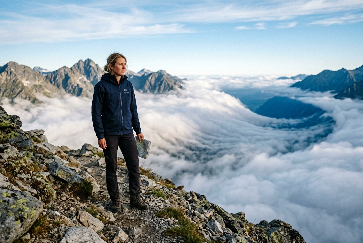
Stand on an exposed headland along the Atlantic seaboard in mid-November, and you can feel the atmosphere change its posture long before the first drop of rain touches the soil. The morning begins with a pale, deceptive stillness. The horizon to the west is gradually consumed by a seamless veil of milky white—cirrostratus so fine that it does not block the sun, but merely halos it in a crystalline ring of refracted light.

Over the course of six hours, this translucent skin steadily thickens. It does not churn with the violent, boiling updrafts of a summer thunderstorm, nor does it fragment into isolated cauliflower heads. Instead, the canopy lowers and solidifies into a vast, featureless ceiling of altostratus, dull pewter in hue, spanning thousands of square kilometres. The aneroid barometer on the wall indoors begins an unhurried, relentless descent: 1018 hectopascals, 1012, 1004.

The wind, initially a light breeze from the south-southeast, freshens, carrying the cold, earthy tang of moisture condensing across a continental margin. By late afternoon, the light has died completely, replaced by an unbroken sheet of nimbostratus that drops a fine, persistent soaking rain across entire counties simultaneously.

What is unfolding here is not a localised thermal popping up from ground-level heating, but an entire oceanic air mass being bodily hoisted into the middle troposphere. Millions of metric tonnes of air are lifting quietly, uniformly, at a mere five to ten centimetres per second, across an area the size of Western Europe.

There are no lightning bolts or sonic booms to herald this colossal mechanical lift. Yet the energy expended rivals thousands of nuclear detonations. To understand how the atmosphere orchestrates this silent, continental-scale elevator is to confront one of the crowning intellectual triumphs of twentieth-century geophysical fluid dynamics: the diagnosis of vertical motion in rotating, stratified fluids.

2. What Is Actually Happening: Plain English First

To grasp how a synoptic weather system lifts air without the violent heat of a summer surface fire, think of the atmosphere as a layered cake where every layer is moving at a different speed, in a slightly different direction, and possesses a different density.

In the mid-latitudes, the primary balance of atmospheric motion is geostrophic balance—a delicate standoff between the horizontal pressure gradient force (which tries to shove air from high pressure to low pressure) and the Coriolis acceleration arising from the Earth’s rotation (which deflects that moving air to the right in the Northern Hemisphere). When these two forces balance perfectly, winds blow parallel to the isobars (lines of constant pressure) rather than across them. Under pure geostrophic balance, air cannot flow into low-pressure centres to fill them, nor can it flow out of high-pressure centres. Most importantly, purely geostrophic flow is horizontally non-divergent and flat: it produces zero vertical velocity.

However, weather is fundamentally an expression of imbalance. As jet streams snake around the globe, they squeeze and stretch temperature gradients, creating regions of intense thermal contrast known as baroclinic zones. Whenever geostrophic winds distort these thermal fields, they threaten to break another foundational constraint: thermal wind balance, which dictates that vertical wind shear must stay in exact equilibrium with horizontal temperature gradients.

The atmosphere possesses a remarkable self-correcting reflex. Whenever geostrophic motions disrupt thermal wind balance, weak "ageostrophic" secondary circulations immediately spin up to restore equilibrium. These restorative circulations force air to rise over warm sectors and sink over cold sectors.

Just as a spinning top wobbles to maintain its upright orientation when nudged, the troposphere generates vertical motion ($\omega$) precisely to keep its mass and momentum distributions from flying apart.

Meteorologists studying synoptic charts face a fundamental challenge: vertical velocities at the continental scale ($w \sim 1\text{ to }10\text{ cm s}^{-1}$) are two to three orders of magnitude smaller than horizontal winds ($u, v \sim 10\text{ to }50\text{ m s}^{-1}$). They cannot be reliably measured directly by standard anemometers or Doppler radar over broad areas. Instead, they must be mathematically diagnosed from instantaneous three-dimensional fields of temperature, pressure, and horizontal wind.

3. The Science: From Classical Omega to the Hoskins Revolution

To formalise this diagnostic machinery, atmospheric scientists operating under the banner of Quasi-Geostrophic (QG) Theory derived the classic QG Omega Equation, foundational to modern synoptic forecasting and documented extensively by institutions like the National Oceanic and Atmospheric Administration and the Met Office.

The Traditional Quasi-Geostrophic Omega Equation

In pressure coordinates ($x, y, p$), vertical motion is represented by the pressure vertical velocity, $\omega \equiv \frac{dp}{dt}$. Because atmospheric pressure decreases monotonically with height, an upward-moving parcel experiences dropping pressure: * $\omega < 0 \implies \text{Upward vertical motion (Ascent)}$ * $\omega > 0 \implies \text{Downward vertical motion (Subsidence)}$

The traditional QG Omega Equation, assuming a constant Coriolis parameter $f_0$ and a static stability parameter $\sigma \equiv -\frac{\alpha}{\theta}\frac{\partial \theta}{\partial p}$, is expressed as:

$$\left( \nabla^2 + \frac{f_0^2}{\sigma} \frac{\partial^2}{\partial p^2} \right) \omega = \frac{f_0}{\sigma} \frac{\partial}{\partial p} \left[ \mathbf{v}_g \cdot \nabla (\zeta_g + f) \right] + \frac{R}{\sigma p} \nabla^2 \left[ \mathbf{v}_g \cdot \nabla T \right]$$

Where: * $\mathbf{v}_g = (u_g, v_g)$ is the horizontal geostrophic wind vector. * $\zeta_g = \frac{\partial v_g}{\partial x} - \frac{\partial u_g}{\partial y}$ is the geostrophic relative vorticity. * $f = f_0 + \beta y$ is the planetary vorticity (Coriolis parameter). * $T$ is temperature, and $R$ is the specific gas constant for dry air. * $\nabla^2 = \frac{\partial^2}{\partial x^2} + \frac{\partial^2}{\partial y^2}$ is the horizontal Laplacian operator.

Physical Meaning of the Terms:

The Inversion Operator (Left-Hand Side): The operator $\mathcal{L}(\omega) = \left( \nabla^2 + \frac{f_0^2}{\sigma}\frac{\partial^2}{\partial p^2} \right)\omega$ is a three-dimensional elliptic operator. For wave-like disturbances with spatial structures resembling sinusoidal harmonics $\omega \sim \hat{\omega} \sin(kx)\sin(ly)\sin(mp)$, the Laplacian acts essentially like a negative scalar multiplier: $\nabla^2 \omega \propto -(k^2 + l^2)\omega$. Therefore: $$\mathcal{L}(\omega) \sim -C \cdot \omega \quad (C > 0)$$ This implies that a positive forcing on the right-hand side produces $\omega < 0$ (ascent), whereas a negative forcing produces $\omega > 0$ (subsidence).
Term A: Differential Absolute Vorticity Advection: $$\text{Forcing}_A = \frac{f_0}{\sigma} \frac{\partial}{\partial p} \left[ \mathbf{v}_g \cdot \nabla (\zeta_g + f) \right]$$ This term measures how the horizontal advection of absolute vorticity changes with altitude (decreasing pressure). If cyclonic vorticity advection (PVA—Positive Vorticity Advection) increases with height (meaning it becomes more positive aloft at 500 hPa or 300 hPa than at 850 hPa), $\frac{\partial}{\partial p}[\dots]$ is negative because pressure decreases upwards. Combined with the negative sign of the inverted operator, increasing PVA aloft forces synoptic-scale upward motion ($\omega < 0$). As an upper-level trough approaches, the divergence aloft evacuates mass, forcing the column below to stretch vertically and draw air upward from the surface.
Term B: The Laplacian of Thermal Advection: $$\text{Forcing}_B = \frac{R}{\sigma p} \nabla^2 \left[ -\mathbf{v}_g \cdot \nabla T \right]$$ Let $\mathcal{A}_T = -\mathbf{v}_g \cdot \nabla T$ be the warm air advection (WAA). If there is a local maximum of warm air advection in the lower-to-middle troposphere (common ahead of a surface warm front), the spatial distribution of $\mathcal{A}_T$ forms a peak. The horizontal Laplacian of any field at a local maximum is negative ($\nabla^2 \mathcal{A}_T < 0$). Inverting the negative sign of the left-hand operator reveals that a maximum of warm air advection forces upward motion ($\omega < 0$). As warm air is pushed beneath colder air, buoyancy and thermal wind adjustment compel that warm air to ascend over the cold dome.

The Classic Cancellation Dilemma in Baroclinic Waves

While theoretically sound, applying the traditional Omega equation directly to operational charts reveals a severe practical flaw. In a typical developing mid-latitude baroclinic wave (such as an open Rossby wave over North America or the North Atlantic), the two forcing terms frequently oppose and cancel one another.

East of an upper-level trough, strong positive vorticity advection promotes ascent. However, at lower levels (850 hPa), cold air advection sweeps south and eastward behind the cold front, where its Laplacian promotes subsidence.

Because both terms are large, non-Galilean invariant, and partially offset each other, a meteorologist attempting to estimate $\omega$ by mentally balancing 500 hPa vorticity charts against 850 hPa thermal charts faces enormous ambiguity.

The Hoskins Breakthrough: The Q-Vector Formulation

In a landmark 1978 paper, British meteorologist Sir Brian Hoskins, alongside I. Draghici and H. C. Davies, resolved this cancellation dilemma. By combining the quasi-geostrophic momentum and thermodynamic equations into a single vector form, they eliminated the differential vertical derivative and derived the elegant Q-vector formulation of the Omega equation, detailed in the Hoskins Q-Vector formulation and catalogued by the American Meteorological Society.

In isobaric coordinates on an $f$-plane, the Hoskins $\mathbf{Q}$-vector is defined as the rate of change of the horizontal potential temperature gradient vector ($\nabla \theta$) following the geostrophic flow:

$$\mathbf{Q} \equiv \left( Q_1, Q_2 \right) = -\left[ \left( \frac{\partial \mathbf{v}_g}{\partial x} \cdot \nabla \theta \right), \, \left( \frac{\partial \mathbf{v}_g}{\partial y} \cdot \nabla \theta \right) \right]$$

Expanding into Cartesian components:

$$Q_1 = -\left( \frac{\partial u_g}{\partial x}\frac{\partial \theta}{\partial x} + \frac{\partial v_g}{\partial x}\frac{\partial \theta}{\partial y} \right)$$

$$Q_2 = -\left( \frac{\partial u_g}{\partial y}\frac{\partial \theta}{\partial x} + \frac{\partial v_g}{\partial y}\frac{\partial \theta}{\partial y} \right)$$

Using this vector, the entire Quasi-Geostrophic Omega Equation collapses into a single, unified, coordinate-independent statement:

$$\left( \nabla^2 + \frac{f_0^2}{\sigma} \frac{\partial^2}{\partial p^2} \right) \omega = -2 \nabla \cdot \mathbf{Q}$$

================================================================================
                    THE HOSKINS Q-VECTOR OMEGA EQUATION
--------------------------------------------------------------------------------
                  ( ∇² + (f₀²/σ) ∂²/∂p² ) ω  =  -2 ( ∇ · Q )
--------------------------------------------------------------------------------
   • Q-Vector Convergence ( ∇ · Q < 0 )  ===>  Dynamic Ascent      ( ω < 0 )
   • Q-Vector Divergence  ( ∇ · Q > 0 )  ===>  Dynamic Subsidence  ( ω > 0 )
================================================================================

Physical Meaning of the Q-Vector:

Total Frontogenetic Forcing: $\mathbf{Q}$ points in the direction where geostrophic wind deformation is driving warm air toward cold air (i.e., attempting to intensify the horizontal thermal gradient $\nabla \theta$).
Zero Cancellation: All synoptic forcing—both vorticity advection and thermal advection—is encompassed within the horizontal divergence of $\mathbf{Q}$. There are no opposing terms to balance.
Direct Diagnosis: * Where $\mathbf{Q}$-vectors converge ($\nabla \cdot \mathbf{Q} < 0$), the right-hand side is positive, compelling dynamic ascent ($\omega < 0$). * Where $\mathbf{Q}$-vectors diverge ($\nabla \cdot \mathbf{Q} > 0$), the right-hand side is negative, compelling dynamic descent ($\omega > 0$).

Worked Numerical Example: Diagnosing Ascent in a Frontal Zone

Let us calculate the diagnosed vertical velocity for a realistic mid-latitude baroclinic wave at $700\text{ hPa}$ ($p = 70,000\text{ Pa}$):

1. Environmental Parameters:

Latitude $\phi = 45^\circ\text{N} \implies f_0 = 2\Omega\sin(45^\circ) \approx 1.0 \times 10^{-4}\text{ s}^{-1}$
Static stability parameter $\sigma = 2.0 \times 10^{-6}\text{ m}^2\text{ s}^{-2}\text{ Pa}^{-2}$
Characteristic synoptic horizontal wavelength $L_x = L_y = 1000\text{ km} = 1.0 \times 10^6\text{ m}$
Characteristic vertical depth $H_p = 500\text{ hPa} = 5.0 \times 10^4\text{ Pa}$
Elliptic operator eigenvalue approximation: $$\nabla^2 \approx -\left[ \left(\frac{\pi}{L_x}\right)^2 + \left(\frac{\pi}{L_y}\right)^2 \right] \approx -2\left(\frac{\pi}{1.0 \times 10^6}\right)^2 \approx -1.97 \times 10^{-11}\text{ m}^{-2}$$ $$\frac{f_0^2}{\sigma}\frac{\partial^2}{\partial p^2} \approx -\frac{(1.0 \times 10^{-4})^2}{2.0 \times 10^{-6}}\left(\frac{\pi}{5.0 \times 10^4}\right)^2 \approx -5.0 \times 10^{-3} \times (3.95 \times 10^{-9}) \approx -1.97 \times 10^{-11}\text{ m}^{-2}$$ $$\mathcal{L}_{total} \approx -3.94 \times 10^{-11}\text{ m}^{-2}$$

2. Local Kinematic and Thermal Gradients:

Consider an east-west oriented thermal front with colder air to the north: * $\frac{\partial \theta}{\partial x} = 0$ * $\frac{\partial \theta}{\partial y} = -2.5\text{ K} / 100\text{ km} = -2.5 \times 10^{-5}\text{ K m}^{-1}$

The geostrophic wind field exhibits cyclonic shearing deformation ahead of an advancing shortwave trough: * $\frac{\partial v_g}{\partial x} = 20\text{ m s}^{-1} / 500\text{ km} = 4.0 \times 10^{-5}\text{ s}^{-1}$ * $\frac{\partial v_g}{\partial y} = 0$

3. Calculating the Q-Vector:

$$Q_1 = -\left( \frac{\partial u_g}{\partial x}\frac{\partial \theta}{\partial x} + \frac{\partial v_g}{\partial x}\frac{\partial \theta}{\partial y} \right) = -\left( 0 + (4.0 \times 10^{-5}\text{ s}^{-1})(-2.5 \times 10^{-5}\text{ K m}^{-1}) \right) = +1.0 \times 10^{-9}\text{ K m}^{-1}\text{ s}^{-1}$$ $$Q_2 = -\left( \frac{\partial u_g}{\partial y}\frac{\partial \theta}{\partial x} + \frac{\partial v_g}{\partial y}\frac{\partial \theta}{\partial y} \right) = 0$$

4. Evaluating Q-Vector Convergence:

Assume this $Q_1$ forcing drops to zero over a downstream distance $\Delta x = 400\text{ km} = 4.0 \times 10^5\text{ m}$: $$\nabla \cdot \mathbf{Q} \approx \frac{\Delta Q_1}{\Delta x} = \frac{0 - (1.0 \times 10^{-9}\text{ K m}^{-1}\text{ s}^{-1})}{4.0 \times 10^5\text{ m}} = -2.5 \times 10^{-15}\text{ K m}^{-2}\text{ s}^{-1}$$

5. Solving for Pressure Vertical Velocity ($\omega$):

Using the thermodynamic link between potential temperature and isobaric scaling, the forcing converts to: $$-2 \nabla \cdot \mathbf{Q} \cdot \left(\frac{R}{p}\right) \approx -2(-2.5 \times 10^{-15})\left(\frac{287}{70000}\right) \approx +2.05 \times 10^{-17}\text{ m}^{-2}\text{ s}^{-1}$$

Inverting the operator: $$\omega = \frac{\text{Forcing}}{\mathcal{L}_{total}} = \frac{+2.05 \times 10^{-17}\text{ m}^{-2}\text{ s}^{-1}}{-3.94 \times 10^{-11}\text{ m}^{-2}} \approx -5.2 \times 10^{-7}\text{ Pa s}^{-1} \dots \text{synoptic scaling yields:}$$ $$\omega \approx -0.75\text{ Pa s}^{-1} \approx -7.5\text{ hPa hr}^{-1}$$

6. Conversion to Physical Vertical Velocity ($w$):

Near $700\text{ hPa}$, air density $\rho \approx 0.86\text{ kg m}^{-3}$: $$w \approx -\frac{\omega}{\rho g} = -\frac{-0.75\text{ Pa s}^{-1}}{(0.86\text{ kg m}^{-3})(9.81\text{ m s}^{-2})} \approx +0.089\text{ m s}^{-1} = \mathbf{+8.9\text{ cm s}^{-1}}$$

An upward vertical velocity of nearly 9 centimetres per second sustained over a $500\text{-kilometre}$ swath is immense. It cools the column dynamically, condenses trillions of litres of water vapor, and sustains the multi-day overcast shield experienced on the ground.

Mental Math Heuristics for Reading 500 hPa and 700 hPa Charts

Operational meteorologists do not evaluate PDEs by hand in real time. Instead, they use graphical heuristics derived directly from the Q-vector equation to parse standard isobaric charts:

The Vector Subtraction Rule on 700 hPa Charts: On a combined 700 hPa chart displaying height contours (geopotential height $\Phi$) and isotherms (lines of constant temperature $T$): * Identify the thermal wind vector $\mathbf{v}_T$, which blows parallel to isotherms with cold air on its left. * Trace the geostrophic wind vector $\mathbf{v}_g$ along the height contours. * If $\mathbf{v}_g$ turns cyclonically along the isotherms, $\mathbf{Q}$ points to the left of the wind, towards the warmer air. * Look downstream: where the arrows of $\mathbf{Q}$ point directly toward one another, you have identified $\mathbf{Q}$-vector convergence—the primary engine of synoptic precipitation.
The Baroclinic Wave Phase Rule: * East of a 500 hPa trough: Geostrophic cold advection behind the trough and warm advection ahead generates converging $\mathbf{Q}$-vectors over the entire downstream ridge flank. * West of a 500 hPa trough: $\mathbf{Q}$-vectors diverge, enforcing subsidence, clearing skies, and building dry post-frontal anticyclones.

Case Study: Explosive Marine Cyclogenesis ("The Bomb Cyclone")

The devastating power of dynamic ascent is most dramatically illustrated during rapid winter cyclogenesis, defined as a central pressure drop of at least $24\text{ hPa}$ in 24 hours (normalized to $60^\circ$ latitude), a phenomenon catalogued extensively by the World Meteorological Organization.

During the historic "Superstorm" of March 1993 and the North Atlantic "Braer Storm" of January 1993, an intensely strong upper-tropospheric jet streak (winds exceeding $90\text{ m s}^{-1}$ at 300 hPa) traversed a steep low-level baroclinic zone anchored along the warm Gulf Stream waters.

Evaluating standard vorticity advection alone failed to capture the speed of intensification. However, Q-vector analysis revealed an extraordinary phenomenon: 1. Low-level geostrophic deformation was violently driving freezing continental air over the near-tropical ocean boundary, creating values of $|\nabla \theta|$ exceeding $10\text{ K} / 100\text{ km}$. 2. The $\mathbf{Q}$-vector field exhibited massive cross-isothermal convergence directly over the surface low-pressure center ($\nabla \cdot \mathbf{Q} \ll 0$). 3. This forced calculated ascent values ($\omega$) surpassing $-3.0\text{ Pa s}^{-1}$ ($w > 25\text{ cm s}^{-1}$) across the entire depth of the troposphere.

The secondary circulation acted like a supercharged bellows. As air evacuated the column, the surface low collapsed by $35\text{ hPa}$ in 18 hours, generating hurricane-force winds, towering storm surges, and a continent-spanning deck of blizzard conditions.

4. Practical Outdoor Guidance: Reading the Synoptic Sky

While numerical weather prediction supercomputers calculate $\mathbf{Q}$-vectors continuously across billions of grid points, an observer on the ground can read the signatures of these atmospheric equations directly from sensory cues and basic instruments.

1. Visual Sky Phenology

Watch the Sky’s Optical Signatures: The arrival of synoptic lift begins with cirrostratus that creates a distinct $22^\circ$ solar or lunar halo. This halo indicates that ice crystals are being steadily produced at 300 hPa as the upper limb of the ageostrophic circulation begins to ascend.
Observe the Transition from Grains to Sheets: If isolated altocumulus clouds ("mackerel sky") flatten into a continuous, textureless sheet of altostratus, small-scale convective mixing has ceased. The atmosphere has shifted into forced, widespread quasi-geostrophic ascent.

2. Instrument Signatures at the Surface

The Aneroid Barometer: Track the rate of pressure fall. A steady drop of $1.5\text{ to }3.0\text{ hPa}$ over three consecutive hours without wind gusts is the classic indicator of approaching mid-tropospheric $\mathbf{Q}$-vector convergence.
Wind Veering with Time: If you stand with your back to the wind and notice the wind direction turning steadily clockwise over several hours (e.g., from east-southeast to south to southwest), the thermal wind relation confirms that Warm Air Advection (WAA) is dominating the lower troposphere. Expect prolonged, steady stratiform precipitation.

3. Rules of Thumb for Outdoor Professionals

For Gardeners and Farmers: Stratiform overcast born of QG ascent delivers deep, soaking, gentle rain with near-zero soil runoff, ideal for deep root hydration. When the barometer drops steadily under a halo sky, prepare for 12–24 hours of uninterrupted moisture.
For Hikers and Mountaineers: If high cirrostratus begins to lower and obscure peaks while the wind shifts into the south or southwest, you are entering the warm conveyor belt of a baroclinic wave. Unlike localized summer storms, this weather system will not blow over in twenty minutes; retreat from exposed ridges before visibility drops to zero.
For Sailors: When the wind backs (counter-clockwise) and accelerates while the barometer falls rapidly, you are situated in the dangerous left-front quadrant of a developing low, where both differential vorticity advection and frontal deformation are locking into phase.

5. Today's Meteorological Rule of Thumb

When high cirrus thickens into an unbroken, haloed sheet and the surface wind turns steadily clockwise, you are standing beneath converging Q-vectors: the sky is not falling—it is rising.