Skew-T Log-P Diagrams & Radiosonde Soundings: Decoding Vertical Atmospheric Profiles for Field Weather Prediction
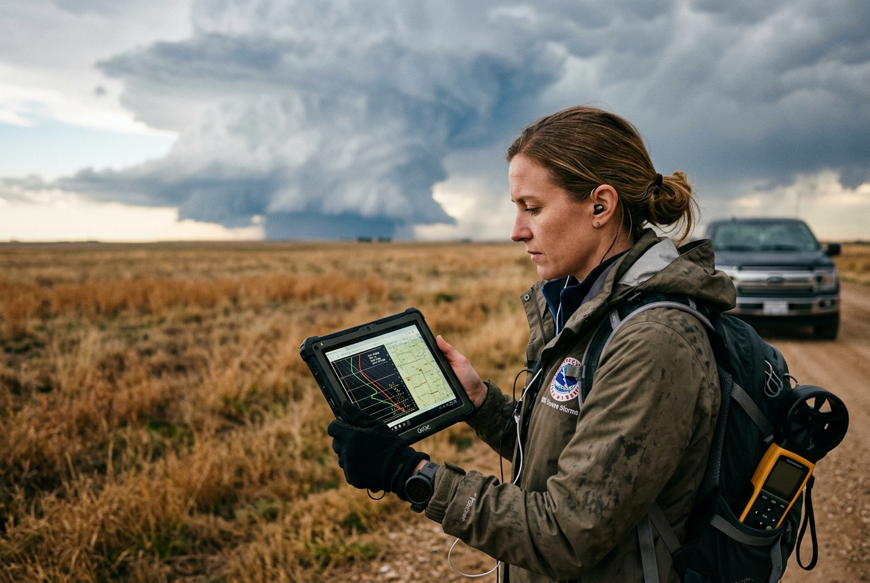
How a two-dimensional thermodynamic chart unlocks the three-dimensional secrets of storm initiation, boundary layer capping, and vertical convective energy.
1. Outdoor Observer Field Notes: The View from the Ground
Stand in an open field on a sultry midsummer afternoon in the mid-latitudes. The air feels oppressive, thick with moisture that clings to your skin. The wind, which blew gently out of the southwest at dawn, has slackened into an ominous, heavy calm. Looking up, the sky presents a deceptive calm: a pale blue canopy crossed by faint wisps of cirrus, underlaid by a hazy layer of flat-topped cumulus clouds drifting low on the horizon. To an untrained observer, it appears to be nothing more than a warm, humid afternoon.
Yet, to an experienced field meteorologist, the atmosphere is vibrating with potential energy. You notice subtle signs: the cumulus clouds are suppressed, their tops flattening out as if striking an invisible ceiling at three thousand feet. This is the visual signature of a capping inversion—a dense layer of warm air sitting atop the boundary layer like a pressure cooker lid. Below this lid, solar radiation continues to cook the Earth's surface, pumping heat and evapotranspirating moisture into a narrowing vertical slice of air.
                                    THE CONVECTIVE LANCE

       Height (z)
           ^
           |              Troposphere Upper Bound / Equilibrium Level (EL)
           |             /
           |            /  [ Anvil Cirrus Spreading ]
           |           /
           |          / |  <-- Free Convection Ascent Path (Moist Adiabat)
           |         /  |
           |        /   |  Positive Area (CAPE)
           |       /    |  (Parcel warmer than Environment)
           |      /     |
           |     LFC    |  <-- Level of Free Convection (Cap Broken!)
           |    [=== CAPPING INVERSION LAYER ===]  <-- Negative Area (CIN)
           |     LCL    |  <-- Lifting Condensation Level (Cloud Base)
           |      |     |
           |      |     |  Unsaturated Ascent (Dry Adiabat)
           |     /      |
       SFC |----/-------+-------------------------------------------> Temperature (T)
               Surface Temp (T_sfc) & Dewpoint (T_d)
As the sun climbs past peak heating, you watch the horizon. A single cumulus tower suddenly breaches the invisible ceiling. Instead of flattening, its head explodes upward in a violently growing turret—a cumulus congestus transforming into a cumulonimbus in a matter of minutes. The cloud top shoots through the mid-troposphere at speeds exceeding thirty meters per second, flaring into a classic anvil profile as it hits the tropopause. The barometric pressure on your pocket altimeter begins a sudden, precipitous drop, followed by a cool, sharp gust of wind smelling faintly of ozone and rain.
What transformed that tranquil afternoon into a localized severe weather outbreak? Ground-level observations—temperature, barometric pressure, and relative humidity—only reveal conditions inside a thin skin of air two meters above the grass. They tell you nothing about the temperature structure three thousand meters up, the dryness of the mid-troposphere, or the strength of the lid holding the storm back. To see the three-dimensional physics of the atmosphere, meteorologists rely on radiosondes: instrumented weather balloons launched twice daily worldwide that measure temperature, pressure, humidity, and wind velocity as they ascend to over thirty kilometers.
When this radiosonde data is plotted on a Skew-T Log-P diagram, it paints an explicit thermodynamic profile of the sky—a atmospheric fingerprint that reveals whether the air will remain tranquil or unleash catastrophic convective storms.
2. Physical Principles & Intuitive Science: The Non-Orthogonal Engine
To understand how a Skew-T Log-P diagram works, we must first examine why conventional Cartesian charts ($X-Y$ graph of Temperature vs. Altitude) fail for atmospheric thermodynamics.
In a standard linear graph, as air rises and expands against decreasing pressure, the work done by or on an air parcel does not correspond to visual geometric area. In classical thermodynamics, energy transformations are analyzed using Clapeyron diagrams ($P-V$ or $T-s$ diagrams), where the area enclosed by a cyclic process on the graph is directly proportional to the physical work done ($W = \oint P \, dV$).
The atmosphere, however, is stratified by pressure ($P$) across orders of magnitude, decreasing exponentially with altitude ($z$). If we plot pressure linearly, the lower atmosphere—where virtually all weather occurs—is compressed into a tiny strip at the bottom of the page, while the stratosphere occupies the upper two-thirds. To expand the troposphere, meteorologists use the logarithm of pressure ($\ln P$) as the vertical axis, oriented so that pressure decreases upward (matching altitude).
   CONVENTIONAL CARTESIAN GRID                 SKEW-T LOG-P GRID
   (Area DOES NOT equal energy)           (Equal area equals equal energy)

P (Pressure)                           ln(P)
   ^                                      ^
   | |  |  |  |                           | \  \  \  \  \ Isotherms skewed 45°
   | |  |  |  |                           |  \  \  \  \  \
   | |  |  |  |                           |   \  \  \  \  \
   +------------> T (Temp)                +-----------------> T (Temp)
However, simply plotting $T$ vs. $\ln P$ creates another problem: as air parcels rise, they cool along lines that slant heavily to the left. On a standard rectangular grid, the environmental temperature profile and rising parcel paths run nearly parallel to one another at steep angles, making it almost impossible to visually measure the small, critical temperature differences between a rising cloud parcel and its surrounding air.
To fix this, Heinrich Stüve and subsequent atmospheric physicists skewed the temperature axis to the right by $45^\circ$. This transformation yields the Skew-T Log-P diagram, an equal-area (isoperimetric) thermodynamic grid. On a Skew-T diagram:
1. Isobars (lines of constant pressure) are horizontal parallel straight lines, scaled logarithmically ($\ln P$).
2. Isotherms (lines of constant temperature) are straight parallel lines slanted upward and to the right at a $45^\circ$ angle.
3. Dry Adiabats (lines of constant potential temperature, $\theta$) curve gently upward to the left. They represent the rate at which unsaturated air cools as it rises due to expansion.
4. Moist (Saturated) Adiabats (lines of constant equivalent potential temperature, $\theta_e$) curve upward, leaning toward the right as height increases. They reflect the cooling rate of saturated air, where the latent heat released by condensing water vapor partially offsets radiative and expansional cooling.
5. Saturation Mixing Ratio Lines ($w_s$) are dashed, gently sloping lines tilted to the right, representing the maximum grams of water vapor one kilogram of dry air can hold at a given temperature and pressure.
Because the grid is mathematically constructed to preserve equal-area energy representation, the physical area enclosed between a parcel ascent curve and the environmental temperature curve is strictly proportional to the kinetic energy gained or lost by the air parcel.
3. Accessible Mathematical Foundations: Deriving the Atmospheric Mechanics
To analyze atmospheric soundings with mathematical rigor, we begin with a simple physical experience and build up to the thermodynamic equations that govern vertical motion.
Step 1: The Bicycle Pump & The Hydrostatic Balance
Have you ever noticed that when you rapidly pump up a bicycle tire, the bottom of the pump becomes hot to the touch? Conversely, when compressed air escapes from an aerosol can, the nozzle gets freezing cold. This is adiabatic temperature change: work done compressing a gas adds thermal energy, while work done by a expanding gas extracts thermal energy, all without exchanging heat with the outside environment ($dq = 0$).
Now consider a slab of air resting in the atmosphere with density $\rho$, cross-sectional area $A$, and vertical thickness $dz$. The upward force on the bottom of the slab due to pressure $P$ must balance the downward force from pressure $P + dP$ at the top plus the weight of the air slab itself:
$$P \cdot A - (P + dP) \cdot A = \rho \cdot A \cdot dz \cdot g$$
Simplifying gives the fundamental Hydrostatic Equation:
$$\frac{dP}{dz} = -\rho g$$
Using the Ideal Gas Law for dry air ($P = \rho R_d T$, where $R_d = 287.05 \text{ J/(kg}\cdot\text{K)}$ is the dry air gas constant), we substitute density $\rho = \frac{P}{R_d T}$ into the hydrostatic equation:
$$\frac{dP}{dz} = -\frac{P g}{R_d T} \implies \frac{dP}{P} = -\frac{g}{R_d T} dz$$
Integrating this differential equation from height $z_1$ to $z_2$ assuming an average layer temperature $\bar{T}$, we derive the classical Hypsometric Equation, referenced in the NOAA Atmospheric Sounding Guidelines:
$$\Delta z = z_2 - z_1 = \frac{R_d \bar{T}_v}{g} \ln\left(\frac{P_1}{P_2}\right)$$
where $T_v$ is the virtual temperature, accounting for the density effect of water vapor. This equation proves that the physical height difference between two pressure surfaces on a Skew-T diagram is proportional to the natural logarithm of the pressure ratio scaled by the absolute temperature.
HYDROSTATIC BALANCE OF AN ATMOSPHERIC SLAB

P + dP  (Lower pressure acting downward)
        v v v v v v v v v v v v
      +-------------------------+
      |  Density = \rho         |
      |  Thickness = dz         | <-- Weight Force = \rho * g * A * dz
      +-------------------------+
        ^ ^ ^ ^ ^ ^ ^ ^ ^ ^ ^ ^
              P     (Higher pressure acting upward)
Step 2: The Dry Adiabatic Lapse Rate ($\Gamma_d$)
When an unsaturated air parcel rises, it expands because ambient atmospheric pressure decreases with height. According to the First Law of Thermodynamics:
$$dq = c_p dT - \alpha dP$$
where $dq$ is heating, $c_p \approx 1004 \text{ J/(kg}\cdot\text{K)}$ is the specific heat of dry air at constant pressure, $dT$ is temperature change, and $\alpha = 1/\rho$ is specific volume.
For an adiabatic process ($dq = 0$), we set $c_p dT = \alpha dP = \frac{1}{\rho} dP$. Substituting the hydrostatic equation ($dP = -\rho g dz$):
$$c_p dT = \frac{1}{\rho} (-\rho g dz) = -g dz$$
Rearranging gives the Dry Adiabatic Lapse Rate ($\Gamma_d$):
$$\Gamma_d = -\frac{dT}{dz} = \frac{g}{c_p} = \frac{9.81 \text{ m/s}^2}{1004 \text{ J/(kg}\cdot\text{K)}} \approx 9.8 \text{ }^\circ\text{C/km} \text{ (or } 9.8 \text{ }^\circ\text{C per 1,000 meters)}$$
This constant slope is depicted on every Skew-T diagram as the solid dry adiabats slanted upward to the left. Unsaturated air will always cool at approximately $10\,^\circ\text{C}$ for every kilometer it rises.
Step 3: Latent Heat & The Moist Adiabatic Lapse Rate ($\Gamma_m$)
Once an air parcel cools to its dewpoint temperature, water vapor condenses into liquid droplets, releasing latent heat of vaporization ($L_v \approx 2.5 \times 10^6 \text{ J/kg}$). This internal heat release counteracts expansional cooling.
The First Law of Thermodynamics for saturated air includes the latent heat term:
$$dq = -L_v dw_s = c_p dT - \alpha dP$$
Through algebraic substitution using the Clausius-Clapeyron relation, we derive the Moist Adiabatic Lapse Rate ($\Gamma_m$):
$$\Gamma_m = -\frac{dT}{dz} = g \cdot \frac{1 + \frac{L_v w_s}{R_d T}}{c_p + \frac{L_v^2 w_s \epsilon}{R_d T^2}}$$
where $w_s$ is the saturation mixing ratio and $\epsilon = \frac{M_{H_2O}}{M_{dry}} \approx 0.622$.
Key Insight: Unlike $\Gamma_d$, the moist lapse rate $\Gamma_m$ is variable. In warm, humid air near the surface, high vapor content releases vast amounts of latent heat, slowing the moist cooling rate to as little as $4\,^\circ\text{C/km}$. In cold polar air or high altitudes, where air holds negligible moisture ($w_s \to 0$), $\Gamma_m$ approaches the dry lapse rate $\Gamma_d \approx 9.8\,^\circ\text{C/km}$.
Step 4: Thermodynamic Energy Integrals (CAPE and CIN)
The primary reason meteorologists use the Skew-T diagram is to compute the net vertical kinetic energy available to accelerate an air parcel upward. This acceleration is governed by buoyancy:
$$a = \frac{d^2z}{dt^2} = g \left( \frac{T_{v,\text{parcel}} - T_{v,\text{env}}}{T_{v,\text{env}}} \right)$$
Integrating this buoyant acceleration over the vertical height interval where the parcel is warmer than its surroundings yields Convective Available Potential Energy (CAPE), measured in Joules per kilogram ($\text{J/kg}$):
$$\text{CAPE} = \int_{z_{\text{LFC}}}^{z_{\text{EL}}} g \left( \frac{T_{v,\text{parcel}}(z) - T_{v,\text{env}}(z)}{T_{v,\text{env}}(z)} \right) dz$$
Using the hydrostatic equation ($dz = -\frac{R_d T_{v,\text{env}}}{g} d(\ln P)$), we transform the spatial integral into a pressure-coordinate area integral on the Skew-T diagram:
$$\text{CAPE} = -R_d \int_{P_{\text{LFC}}}^{P_{\text{EL}}} \left( T_{v,\text{parcel}} - T_{v,\text{env}} \right) d(\ln P)$$
                               CAPE & CIN ENERGY INTEGRALS

Log Pressure (ln P)
       ^
       |           /
  P_EL +----------/--------------------- Equilibrium Level (Top of Positive Area)
       |         /  :
       |        /   :
       |       /    :   POSITIVE AREA (CAPE)
       |      /     :   Integration of (T_parcel - T_env) > 0
       |     /      :   Parcel accelerates upward rapidly!
  P_LFC+----+-------+------------------- Level of Free Convection
       |    | CAP   |   NEGATIVE AREA (CIN)
       |    | (CIN) |   Work required to lift parcel over the cap!
  P_SFC+----+-------+------------------- Surface
       +----------------------------------> Temperature (T)
The theoretical maximum vertical velocity ($w_{\max}$) achievable by an updraft inside a thunderstorm cell can be derived directly from CAPE by equating kinetic energy to potential energy ($\frac{1}{2} w^2 = \text{CAPE}$):
$$w_{\max} = \sqrt{2 \cdot \text{CAPE}}$$
For example, a sounding with a CAPE of $3,200 \text{ J/kg}$ yields a theoretical maximum updraft velocity of $w_{\max} = \sqrt{2 \cdot 3200} = 80 \text{ m/s} \approx 288 \text{ km/h}$, easily capable of supporting giant hail.
4. Step-by-Step Graphical Construction of Key Convective Indices
To evaluate a raw radiosonde sounding in the field, meteorologists follow a precise geometric construction sequence on the Skew-T chart.
=================================================================================
                 GRAPHICAL CONSTRUCTION FLOWCHART ON A SKEW-T
=================================================================================

[ Surface Air Temp (T) ]                 [ Surface Dewpoint (T_d) ]
             |                                         |
             v                                         v
   Follow DRY ADIABAT up                   Follow MIXING RATIO LINE up
             \                                         /
              \                                       /
               +------------------> INTERSECTION <---+
                                        |
                                        v
                       LIFTING CONDENSATION LEVEL (LCL)
                                 (Cloud Base)
                                        |
                                        v
                           Follow MOIST ADIABAT up
                                        |
            +---------------------------+---------------------------+
            |                                                       |
            v                                                       v
  Intersects Env Temp Profile                             Crosses Env Temp Profile
    (T_parcel < T_env)                                      (T_parcel > T_env)
            |                                                       |
            v                                                       v
 CONVECTIVE INHIBITION (CIN)                               LEVEL OF FREE CONVECTION (LFC)
      (Negative Area)                                         (Free Acceleration Begins)
                                                                    |
                                                                    v
                                                          Follow MOIST ADIABAT up
                                                                    |
                                                                    v
                                                          Crosses Env Temp Profile
                                                            (T_parcel = T_env)
                                                                    |
                                                                    v
                                                         EQUILIBRIUM LEVEL (EL)
                                                             (Anvil Top)
=================================================================================
1. Lifting Condensation Level (LCL)
The LCL represents the exact pressure height where an unsaturated air parcel, lifted mechanically from the surface, becomes saturated and cloud droplets begin to condense.
* Graphical Method:
1. Identify surface air temperature ($T$) and surface dewpoint ($T_d$).
2. From $T$, construct a path upward along the solid Dry Adiabat.
3. From $T_d$, construct a path upward along the dashed Saturation Mixing Ratio Line.
4. The point of intersection is the LCL. The pressure at this point marks the visual base of convective clouds.
2. Level of Free Convection (LFC)
The LFC is the height above which a lifted air parcel becomes warmer (less dense) than its surrounding ambient environment, allowing it to rise freely due to positive thermal buoyancy without further external mechanical forcing.
* Graphical Method:
1. From the LCL, continue tracking the parcel upward along the saturated Moist Adiabat.
2. At first, the parcel may remain colder than the surrounding environmental temperature profile ($T_{\text{parcel}} < T_{\text{env}}$)—this layer is the Capping Inversion, generating Convective Inhibition (CIN).
3. The exact altitude where the moist adiabat crosses to the right of the environmental temperature profile ($T_{\text{parcel}} > T_{\text{env}}$) is the LFC.
3. Equilibrium Level (EL)
The EL (often called the neutral buoyancy level) marks the top of the convective storm column, where a rising parcel cools back to match the environmental temperature.
* Graphical Method:
1. Continue following the moist adiabat upward from the LFC through the deep troposphere.
2. The parcel remains warmer than the environment across the positive area (CAPE region).
3. As the parcel approaches the cold tropopause, the environmental profile flattens out while the parcel continues to cool. The altitude where the moist adiabat crosses back to the left of the environmental profile is the EL.
4. This altitude dictates the height of the thunderstorm's spreading anvil cirrus cloud top.
4. Downdraft CAPE (DCAPE) & Microburst Hazard Analysis
While CAPE measures updraft strength, DCAPE quantifies the maximum energy available to produce destructive downward windstorms (microbursts and cold-pool outflow boundaries).
                 DOWNDRAFT CAPE (DCAPE) MECHANISM

Height
    ^
    |    Min \theta_e Air (Mid-Troposphere, ~600-700 hPa)
    |          |
    |          v  [ Rain falls into dry air layer ]
    |          |  [ Evaporative cooling cools parcel ]
    |          |
    |          v  Descends along MOIST ADIABAT to surface
    |         /
    |        /    DCAPE Area (Parcel Colder than Environment)
    |       /     Dense, cold air accelerates downward!
    |      /
    +-----+------------------------------------------------> Temp
        Surface Impactor! (Severe Downburst Gusts > 60 knots)
- Physical Process: Rain drops falling through dry air in the mid-troposphere (typically between $700 \text{ hPa}$ and $500 \text{ hPa}$) evaporate, absorbing latent heat and rapidly cooling the air. This cooled air becomes much denser than the surrounding ambient air and plummets toward the ground.
- Graphical Method:
1. Inspect the sounding between $700 \text{ hPa}$ and $500 \text{ hPa}$ to find the height of the minimum equivalent potential temperature ($\theta_{e,\min}$).
2. From this point, trace down along a moist adiabat down to the surface pressure level.
3. The area enclosed between this moist adiabatic descent path and the environmental profile down to the surface represents DCAPE.
4. Diagnostic Scale: DCAPE values exceeding $1,000 \text{ J/kg}$ indicate a severe threat for destructive downbursts capable of snapping trees and downing powerlines.
5. Actionable Real-World Observational Techniques for Severe Weather Forecasting
Field meteorologists do not evaluate sounding parameters in isolation; they synthesize them to anticipate severe storm initiation, storm mode, and heavy precipitation potential.
+-----------------------------------------------------------------------------------+
|                        SEVERE WEATHER SOUNDING ARCHETYPES                         |
+-----------------------------------------------------------------------------------+
|  1. THE "LOADED GUN" SOUNDING           |  2. THE "ELEVATED MIXED LAYER" (EML)    |
|  - Strong cap (CIN > 100 J/kg)          |  - Deep dry adiabatic lapse rate aloft  |
|  - High surface moisture (w > 14 g/kg)  |  - Originates over arid plateaus        |
|  - Massive CAPE (> 3000 J/kg)           |  - Extremely high instability potential |
|  - Trigger: Surface heating / Front     |  - Prevents premature weak convection   |
+-----------------------------------------------------------------------------------+
A. Evaluating the Capping Inversion ("The Lid")
A capping inversion appears on a Skew-T diagram as a layer where temperature increases with height ($\frac{dT}{dz} > 0$), creating a prominent notch leaning to the right.
- The Loaded Gun Profile: Counterintuitively, the most destructive supercell storms require a strong capping inversion early in the day. The cap acts as a thermal valve: it prevents small, weak updrafts from venting boundary layer heat into the upper atmosphere. Heat and moisture build up beneath the cap all morning.
- Cap Breaking Mechanisms: For severe storms to launch, the cap must be breached before solar heating wanes. Forecasters monitor four primary cap-breaking triggers:
1. Surface Diurnal Heating: Solar radiation increases surface temperature $T_s$, shifting the surface dry adiabat rightward until CIN shrinks to zero.
2. Low-Level Moisture Advection: Dewpoint increases, raising the LCL and lowering the LFC height.
3. Synoptic Dynamic Lifting: Broad-scale ascent ahead of an upper-level trough lifts the entire capping layer, cooling it adiabatically and eroding the inversion.
4. Mesoscale Convergence Lines: Sea breeze fronts, drylines, or thunderstorm outflow boundaries mechanically force air parcels past the LFC.
B. Elevated Mixed Layers (EML)
An Elevated Mixed Layer is an intense thermodynamic feature responsible for major severe weather outbreaks. It forms when air over an elevated, dry plateau (such as the Mexican Plateau or the US High Plains) is intensely heated, generating a deep dry-adiabatic boundary layer. Synoptic winds then transport this warm, dry air layer eastwards over a cool, moist maritime boundary layer (e.g., from the Gulf of Mexico or the Mediterranean).
On a Skew-T diagram, an EML stands out as a thick mid-level layer (between $850 \text{ hPa}$ and $500 \text{ hPa}$) where the environmental temperature curve runs strictly parallel to the dry adiabats ($\frac{dT}{dz} \approx 9.8\,^\circ\text{C/km}$). This exceptionally steep lapse rate aloft maximizes the area between the rising parcel curve and the ambient air, driving CAPE values to extreme levels ($>4,000 \text{ J/kg}$).
C. Precipitable Water Depth (PWAT)
To forecast flash flooding versus dry convective downbursts, meteorologists calculate the total moisture integrated through the vertical atmospheric column—the Precipitable Water (PWAT) depth.
Mathematically, PWAT is expressed as:
$$\text{PWAT} = \frac{1}{\rho_w g} \int_{P_{\text{top}}}^{P_{\text{sfc}}} q \, dP$$
where $q$ is the specific humidity in $\text{kg/kg}$, $\rho_w = 1000 \text{ kg/m}^3$ is liquid water density, and $g = 9.81 \text{ m/s}^2$.
PRECIPITABLE WATER DIAGNOSTIC MATRIX

PWAT Value           Atmospheric Regime            Severe Risk Profile
  -----------------------------------------------------------------------------------
  < 15 mm (0.6 in)     Dry Continental Air           Fire weather; negligible storm risk
  15 – 30 mm           Moderate Humidity             Standard seasonal thunderstorm risk
  30 – 50 mm           Subtropical Moisture Air      Severe wet thunderstorms & downbursts
  > 50 mm (2.0 in)     Tropical Air Mass / Atmospheric River  Extreme Flash Flood Hazard
Forecasters inspect the dewpoint depression ($T - T_d$) across the vertical sounding on the Skew-T chart. If $T$ and $T_d$ lines are almost touching from the surface up to $300 \text{ hPa}$, the sounding is sub-saturated, signaling high precipitation efficiency and extreme flash flooding danger. Conversely, a wide gap between $T$ and $T_d$ in the lower-to-mid troposphere (an "Inverted-V" profile) signals dry air prone to evaporative cooling, raising the hazard rating for high-impact downbursts.
6. Practical Weather Forecasting & Outdoor Guidance
For outdoors enthusiasts, mountaineers, pilots, and field observers, understanding thermodynamic soundings transforms raw weather forecasts into actionable safety decisions.
       SUMMARY SOUNDING CHART: QUICK FIELD INTERPRETATION GUIDE

Key Feature on Skew-T         Physical Meaning                 Outdoor Impact
  ===================================================================================
  Large Negative Area (CIN)     Strong Capping Inversion         No rain early; explosive
                                                                 storms if cap breaks.
  -----------------------------------------------------------------------------------
  Steep Lapse Rate aloft        Deep unstable air layer (EML)    High potential for large
  (T line parallel to Dry Adiabat)                               hail & strong updrafts.
  -----------------------------------------------------------------------------------
  Inverted 'V' shape at base    Very dry low-level air mass      Severe dry microbursts &
  (Wide T - T_d gap near ground)                                 sudden gust fronts.
  -----------------------------------------------------------------------------------
  T and T_d touch up to top     Deeply saturated atmosphere      Torrential rain, low cloud
                                                                 ceilings, flash flooding.
Real-World Field Decision Workflow
-
Pre-Trip Planning (Morning Sounding Check):
* Access the morning $0000\text{Z}$ or $1200\text{Z}$ sounding from authoritative outlets such as the NOAA Storm Prediction Center Sounding Archive or the Met Office Weather Observation Network.
* Check the LCL height: If the LCL is low ($<800 \text{ m}$ above ground) and relative humidity is high, mountain ridge lines will be enveloped in dense cloud base early in the day.
* Check CAPE vs. CIN: A CAPE $>1,500 \text{ J/kg}$ combined with a CIN $<25 \text{ J/kg}$ means thunderstorms will initiate quickly once solar heating reaches the convective temperature ($T_c$). Plan to clear exposed peaks or open water before early afternoon. -
Mid-Day Field Observation:
* Observe cumulus cloud development. Flat, squashed cloud bases reflect an intact capping inversion.
* If cloud tops begin to bulge upward vertically (forming cumulus congestus towers with crisp, cauliflower-like margins), the cap is failing. Free convection has begun. -
Aviation & Flying Safety:
* Pilots check sounding temperature gradients to identify the freezing level ($0\,^\circ\text{C}$ isotherm cross point) and regions of high relative humidity where airframe icing will occur.
* Glider pilots examine the height of the dry lapse rate from the surface to identify the maximum depth of thermal updraft columns.
7. Meteorological Rules of Thumb
🌤️ TODAY'S METEOROLOGICAL RULE OF THUMB
The $10\,^\circ\text{C}$ Rule for Cloud Base (LCL Estimation):
To estimate the height of convective cloud bases ($z_{\text{LCL}}$ in feet) in the field without a chart, measure the surface temperature ($T_{\text{sfc}}$) and dewpoint ($T_{d,\text{sfc}}$) in degrees Celsius:
$$z_{\text{LCL}} \approx (T_{\text{sfc}} - T_{d,\text{sfc}}) \times 400 \text{ feet}$$
(Example: If $T = 30\,^\circ\text{C}$ and $T_d = 18\,^\circ\text{C}$, Spread $= 12\,^\circ\text{C}$. Base $\approx 12 \times 400 = 4,800 \text{ ft AGL}$.)The Hail Threat Threshold:
If CAPE in the hail growth zone (the temperature band between $-10\,^\circ\text{C}$ and $-30\,^\circ\text{C}$ on the Skew-T chart) exceeds $500 \text{ J/kg}$, updrafts will freeze supercooled water into severe, large-diameter hail.The Microburst Alert (Inverted-V):
When the dewpoint depression ($T - T_d$) at the surface exceeds $20\,^\circ\text{C}$ while mid-level moisture remains present, expect severe convective downbursts with minimal rain reaching the ground (dry microbursts).Cap Breakdown Condition:
A capping inversion will fail via thermal heating alone when the surface forecast maximum temperature exceeds the Convective Temperature ($T_c$)—found on the Skew-T by following the moist adiabat from the LFC down to the surface pressure along the dry adiabat.
8. Authoritative Meteorological Resources & Further Reading
To deepen your practical understanding of atmospheric thermodynamics, radiosonde data interpretation, and observational forecasting, consult these reference repositories:
- NOAA Storm Prediction Center Sounding Analysis Page: Live radiosonde soundings across North America featuring real-time Skew-T calculations and convective parameters.
- World Meteorological Organization (WMO) Observing Systems: International standards on radiosonde telemetry, vertical profile sounding techniques, and global upper-air observation networks.
- Met Office Observation Data & Soundings Profile: High-resolution upper-air observational datasets and weather profile modeling documentation.
- Wikipedia Skew-T Log-P Diagram Reference: Detailed mathematical background on non-orthogonal coordinate transformations and thermodynamic chart derivations.
- MIT OpenCourseWare - Atmospheric Thermodynamics & Convection: University lecture notes, hydrostatic equations, and thermodynamic proofs from the Massachusetts Institute of Technology.