Frontogenesis & Slope Gradients: Calculating Air Mass Boundaries for Field Weather Prediction
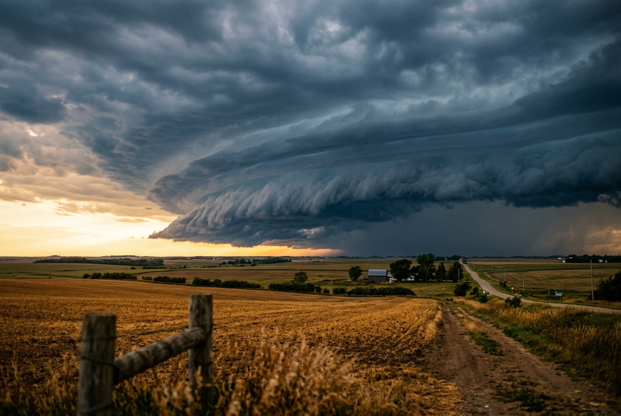
METEOROLOGICAL FIELDWORK | READING THE BARIC SKY
1. Outdoor Observer Field Notes: Reading the Skies and the Barometer
To an experienced outdoor observer, the atmosphere is never static; it is a fluid canvas governed by thermodynamics and motion. Long before a weather front arrives on a synoptic surface chart, subtle clues manifest across the horizon, in the rising of micro-breezes, and on the face of an altimeter-barometer. Understanding how to read air mass boundaries begins not with computer models, but with direct field observations of pressure tendencies, wind vectors, and cloud family evolutions.
Imagine standing on an exposed ridge on an early autumn afternoon. The morning was clear, cold, and still. By noon, however, thin, wispy strands of cirrus (cirrus uncinus, often called "mares' tails") stretch across the upper troposphere from the west. These high-altitude ice-crystal clouds—positioned 8 to 12 kilometers above sea level—are the vanguards of an approaching warm frontal system. Over the next six to twelve hours, as warm, moist air aloft glides over the colder, denser surface air mass, the sky progressively thickens. The cirrus merges into a uniform, translucent sheet of cirrostratus, creating a distinct halo around the sun or moon via the light refraction of hexagonal ice crystals. As the frontal surface tilts lower toward the observer, clouds lower and thicken into mid-level altostrata, obscuring the sun into a pale, diffuse disk. Finally, dark, featureless nimbostratus clouds cap the sky, bringing steady, continuous precipitation.
       TYPICAL WARM FRONTAL CLOUD EVOLUTION (SLOPE ~ 1:200 to 1:400)

Warm Air Mass (Ascending) ----------------------------->
-------------------------------------------------------------------->
                       Altostratus           Cirrostratus      Cirrus
     Nimbostratus    (2,000 - 6,000 m)     (6,000 - 8,000 m)  (>8,000 m)
   (Surface to 2km)      [===]                 [---]            [~ ~ ~]
   ================================------------------------------------
Cold Air Mass (Denser, Wedged Below)
-------------------------------------------------------------------->
Conversely, an approaching cold front presents a far more dramatic and rapid transformation. Rather than a prolonged sequence over hundreds of kilometers, a active cold front acts like a atmospheric snowplow. An observer will notice a falling barometer accompanied by a warm, humid breeze from the south or southwest. On the horizon, a dark wall of clouds emerges: low-level stratocumulus quickly gives way to towering cumulonimbus arcus (shelf clouds). As the boundary sweeps overhead, the surface wind shifts violently—a phenomenon known as a wind shift vector. In the Northern Hemisphere, this shift typically manifests as a rapid "veering" from south-southwesterly to north-northwesterly. Simultaneously, the barometric pressure reaches its absolute minimum right at the trough line before spiking sharply upward, accompanied by a steep drop in dry-bulb temperature and dew point.
Tracking these surface indicators requires a systematic log of three core parameters:
1. Barometric Pressure Tendency ($\Delta P / \Delta t$): A steady decline over 3 hours indicates an approaching synoptic trough; a sudden, rapid rise signals the passage of a cold front boundary.
2. Surface Wind Shift Vectors: Measuring both directional rotation (veering vs. backing) and gust intensity across the boundary.
3. Cloud Morphology Transitions: Mapping the structural shift from stratiform sequence (warm front) or convective vertical towers (cold front).
ATMOSPHERIC DYNAMICS | DENSITY DISCONTINUITIES AND FRONTOGENESIS
2. Physical Principles & Intuitive Science: Atmospheric Mechanisms
To understand why weather fronts form, we must examine the concept of an air mass. An air mass is an immense body of air, spanning thousands of square kilometers, possessing relatively uniform temperature and moisture characteristics acquired over its source region—such as the frozen plains of Arctic Canada (Continental Polar, $cP$) or the equatorial waters of the Gulf of Mexico (Maritime Tropical, $mT$).
When these distinct air masses are brought into proximity by large-scale atmospheric currents, they do not mix instantly. Because air density is inversely proportional to temperature (and modified by moisture), warm air is lighter and more buoyant than cold air. The narrow transition zone separating two contrasting air masses is defined as a meteorological front.
                           COLD FRONT BOUNDARY (SLOPE ~ 1:50 to 1:100)

               Cumulonimbus
                 (Anvil)
                   ||             Warm Air Mass
                   ||             (Forced Upward)
                   ||                  ^ /
                   ||                 / /
      Anvil Head   ||                / /
      ===========\ ||               / /
                  \||              / /
                   ||             / /
  Cold Dense Air   ||            / /
  (Steep Wedge)    ||           / /
  ================>||__________/ /____________________________________
The life cycle of these boundaries—their creation, intensification, and decay—is governed by frontogenesis and frontolysis. Frontogenesis is the process by which horizontal temperature gradients ($\nabla T$) are intensified by atmospheric deformation fields. In synoptic meteorology, this is driven by horizontal shearing and stretching deformation in the wind field. When confluent flow presses isothermal lines closer together, the horizontal thermal gradient steepens dramatically:
$$\text{Frontogenesis Function: } F = \frac{D}{Dt} |\nabla T| > 0$$
For deeper reading on deformation fields and atmospheric kinematics, consult resources provided by the National Oceanic and Atmospheric Administration (NOAA) and the World Meteorological Organization (WMO).
Why do fronts tilt rather than remaining vertical or flattening horizontally? The answer lies in the balance between gravity and Earth's rotation (the Coriolis force). In a non-rotating system, a cold air mass pushed against a warm air mass would slide beneath it until the boundary became completely horizontal, with the dense cold air underneath and warm air on top. However, because Earth rotates, fluids moving across its surface experience a deflection proportional to their velocity and latitude.
As cold air wedges under warm air, the horizontal pressure gradient force generated by the density contrast is balanced by the difference in Coriolis forces acting on the geostrophic winds on either side of the front. This dynamic equilibrium creates a tilted boundary angle, known as the frontal slope.
MATHEMATICAL METEOROLOGY | SLOPE EQUATIONS AND LIFT DYNAMICS
3. Accessible Mathematical Foundations: Margules' Equation & Motion Dynamics
To analyze frontal slopes mathematically, we look to the foundational work of Austrian meteorologist Max Margules, who derived the theoretical slope of a stable density boundary in a rotating fluid frame in 1906. For comprehensive theoretical background, reference the MIT OpenCourseWare Atmospheric Dynamics collection and Wikipedia's guide on Frontogenesis.
Step 1: Intuitive Physical Analogy
Think of oil and water inside a transparent container on a spinning turntable. Water is denser than oil. If the container is static, the oil floats on top in a flat, horizontal layer. But if you spin the container at a constant angular speed, the centrifugal force tilts the interface into a curved slope. In the atmosphere, Earth's rotation plays the role of the turntable, while cold and warm air masses act like water and oil.
Step 2: Margules' Equation for Frontal Slope ($\tan \alpha$)
Margules established that for a sharp, zero-order discontinuity separating two air masses of uniform densities $\rho_1$ (warm) and $\rho_2$ (cold), with mean absolute temperatures $T_1$ and $T_2$, the tangent of the slope angle $\alpha$ is given by:
$$\tan \alpha = \frac{f}{g} \left( \frac{\rho_2 v_1 - \rho_1 v_2}{\rho_1 - \rho_2} \right)$$
Using the ideal gas law ($P = \rho R T$) and assuming hydrostatic balance, Margules' equation is commonly expressed in terms of temperature and geostrophic wind components parallel to the front ($v_{g1}$ and $v_{g2}$):
$$\tan \alpha \approx \frac{f}{g} \bar{T} \left( \frac{v_{g2} - v_{g1}}{T_2 - T_1} \right) = \frac{f}{g} \frac{\bar{T}}{\Delta T} \Delta v_g$$
Where:
* $\alpha$ = Angle of the frontal slope relative to the horizontal surface.
* $f = 2\Omega \sin\phi$ = Coriolis parameter (where $\Omega = 7.292 \times 10^{-5} \text{ rad/s}$ is Earth's angular velocity and $\phi$ is latitude).
* $g$ = Acceleration due to gravity ($9.81 \text{ m/s}^2$).
* $\bar{T}$ = Mean absolute temperature of the two air masses in Kelvin: $\frac{T_1 + T_2}{2}$.
* $\Delta T = T_2 - T_1$ = Temperature difference across the boundary ($K$ or $^\circ C$).
* $\Delta v_g = v_{g2} - v_{g1}$ = Cross-frontal shear in geostrophic wind velocity parallel to the front ($\text{m/s}$).
Step-by-Step Worked Example 1: Calculating Frontal Slope ($\tan \alpha$)
Let us calculate the slope angle of a cold front at latitude $\phi = 45^\circ \text{ N}$.
Given Parameters:
1. Latitude $\phi = 45^\circ \text{ N}$
$$f = 2 (7.292 \times 10^{-5}) \sin(45^\circ) = 1.031 \times 10^{-4} \text{ s}^{-1}$$
2. Gravitational acceleration $g = 9.81 \text{ m/s}^2$
3. Temperature of Warm Air Mass ($T_1$) = $15^\circ \text{C} = 288.15 \text{ K}$
4. Temperature of Cold Air Mass ($T_2$) = $5^\circ \text{C} = 278.15 \text{ K}$
$$\Delta T = T_2 - T_1 = -10 \text{ K} \quad \implies |\Delta T| = 10 \text{ K}$$
$$\bar{T} = \frac{288.15 + 278.15}{2} = 283.15 \text{ K}$$
5. Parallel Geostrophic Wind in Warm Air ($v_{g1}$) = $+5 \text{ m/s}$ (South-to-North)
6. Parallel Geostrophic Wind in Cold Air ($v_{g2}$) = $-15 \text{ m/s}$ (North-to-South)
$$\Delta v_g = v_{g2} - v_{g1} = -15 - 5 = -20 \text{ m/s}$$
Calculation:
$$\tan \alpha = \frac{1.031 \times 10^{-4}}{9.81} \times \frac{283.15}{10} \times 20$$
$$\tan \alpha = (1.051 \times 10^{-5}) \times 28.315 \times 20$$
$$\tan \alpha = 0.005952 \approx \frac{1}{168}$$
Interpretation:
The frontal slope gradient is approximately 1:168 (or roughly 1 km vertical rise for every 168 km horizontal distance). This steep slope is characteristic of a active cold front, driving strong vertical lift. Warm fronts, by comparison, feature much flatter slopes ranging from 1:300 to 1:400.
Step-by-Step Worked Example 2: Calculating Frontal Speed and Ascent Rate
Next, let us derive the propagation velocity of the frontal line and the resulting forced vertical velocity ($w$) of the warm air mass being lifted over it.
Given Parameters:
1. Frontal slope $\tan \alpha = 1:100 = 0.01$
2. Normal wind velocity of the advancing cold air mass perpendicular to the front ($u_n$) = $15 \text{ m/s}$ ($54 \text{ km/h}$)
3. Calm warm air mass ahead of the front ($u_{warm} \approx 0 \text{ m/s}$)
Calculation of Forced Ascent Velocity ($w$):
The rate of forced mechanical lift ($w_{lift}$) experienced by warm air impinging on the moving wedge is calculated by:
$$w_{lift} = u_n \cdot \tan \alpha$$
$$w_{lift} = 15 \text{ m/s} \times 0.01 = 0.15 \text{ m/s} = 15 \text{ cm/s}$$
While 15 cm/s may seem modest, across a synoptic area this persistent vertical motion raises air parcels by $540 \text{ meters per hour}$.
If the ambient warm air is unstable or conditionally unstable—possessing positive Convective Available Potential Energy (CAPE)—this initial mechanical lift easily overcomes the Convective Inhibition (CIN) layer, forcing parcels to their Level of Free Convection (LFC).
                                  BUOYANCY LIFT & CAPE DYNAMICS

  Altitude (z)
       ^
       |          Parcel Path (Moist Adiabat)  / Environment Profile
       |                                      /
       |                                     /  [Free Convection Zone]
       |                                    / /
       |                                   / /
  LFC  |----------------------------------x /  <-- (Mechanical Lift Needed)
       |                                 / /
       |                                / /   [CIN Layer]
       |                               / /
Surface|______________________________/ /__________________________________> Temperature (T)
The net vertical acceleration ($a_z$) above the LFC is governed by the atmospheric buoyancy equation:
$$a_z = \frac{dw}{dt} = g \left( \frac{T_{v,\text{parcel}} - T_{v,\text{env}}}{T_{v,\text{env}}} \right)$$
Where $T_v$ is the virtual temperature accounting for moisture. If the parcel remains $3\text{ K}$ warmer than its environment at $500 \text{ hPa}$ ($\sim 5,500\text{ m}$):
$$a_z = 9.81 \times \left( \frac{3}{250} \right) = 0.1177 \text{ m/s}^2$$
Over a 500-second vertical ascent through the unstable layer, updraft speeds can accelerate from $0.15 \text{ m/s}$ to:
$$w_{final} = w_0 + a_z \cdot t = 0.15 + (0.1177 \times 500) \approx 59 \text{ m/s} \quad (\sim 212 \text{ km/h})$$
This explosive vertical velocity converts moisture into severe convective precipitation, cloud electrification (lightning), and severe thunderstorm downdrafts.
FIELD APPLICATION | SYNOPTIC CHART ANALYSIS AND OUTDOOR SAFETY
4. Practical Weather Forecasting & Outdoor Guidance
Translating theoretical frontogenesis into field awareness is an essential skill for outdoor leaders, mountaineers, mariners, and pilots. Weather forecasts often update every few hours, but localized terrain dynamics can accelerate or retard frontal movement. By linking map-reading to real-time observations, individuals can make informed safety decisions. For real-time updates and field guidance tools, refer to the UK Met Office.
                      SYNOPTIC CHART SYMBOLOGY AND FRONT IDENTIFICATION

      COLD FRONT:                       WARM FRONT:                      OCCLUDED FRONT:
      Blue line with triangles          Red line with semi-circles       Purple line with alternating
      pointing in motion direction      pointing in motion direction     triangles & semi-circles

       ----▲-----▲-----▲----             ----●-----●-----●----            ----▲-----●-----▲---->
1. Reading Surface Synoptic Charts
When examining a surface weather map:
* Isobar Kinks: Fronts reside in troughs of low pressure. Isobars bend sharply away from the low-pressure center when crossing a front.
* Temperature & Dew Point Packaging: Dense clustering of isotherms indicates an active frontogenetic zone. A sharp drop in dew point behind a front signifies dry, cold continental polar air replacing moist marine air.
* Frontal Movement Rule: A front moves at roughly $70\%$ to $80\%$ of the geostrophic wind component perpendicular to the front line measured on the chart.
2. Field Navigation & Safety Strategies
| Phase | Observed Barometric / Sky Sign | Meteorological Reality | Action / Risk Strategy |
|---|---|---|---|
| Pre-Frontal Warm Sector | Falling pressure ($>1.5\text{ hPa/3h}$); warm winds from S/SW; high cirrus thickening to altostratus. | Approaching boundary; thermal advection active; height of ceiling dropping. | Calculate distance to boundary. Secure camp, plan descent routes if in alpine zones. |
| Frontal Line Passage | Minimum pressure spike; sudden wind veering (SW to NW); dense squall line or heavy stratiform rain. | Direct frontal convergence; peak mechanical lift; potential lightning/wind shear. | Seek immediate shelter away from ridges, exposure, or high trees. Suspend water crossings. |
| Post-Frontal Sector | Rapid pressure rise; sharp temperature drop; clear, crisp air with scattered cumulus. | Cold air advection ($CAA$); air mass stabilization; high visibility. | Resume activity, but prepare for colder temperatures and low freezing levels. |
5. Takeaway Box: Today's Meteorological Rule of Thumb
[!IMPORTANT]
METEOROLOGICAL RULE OF THUMB: THE FRONTAL EQUILIBRIUM & WIND SHIFT LAW
Margules' Slope Gradient Standard: Cold fronts feature steep slopes ($\approx 1:50 \text{ to } 1:100$), driving rapid mechanical lift and intense, short-lived convective squalls. Warm fronts feature shallow slopes ($\approx 1:200 \text{ to } 1:400$), creating prolonged stratiform cloud and rain shields spanning hundreds of kilometers.
Buys Ballot's Wind Shift Law: Standing with your back to the wind in the Northern Hemisphere, low pressure is to your left. When a cold front passes, the wind veers (rotates clockwise, e.g., South-West to North-West). A counter-clockwise shift (backing) indicates an approaching warm advection sector or passing secondary low.
The 3-Hour Barometric Tendency Warning: A steady drop in surface pressure exceeding $3 \text{ hPa}$ within 3 hours is a reliable indicator of an approaching front or squall line. Immediate safety protocols should be activated in exposed terrain.
Key Equation Summary:
$$\text{Frontal Slope: } \tan \alpha \approx \frac{f}{g} \frac{\bar{T}}{\Delta T} \Delta v_g \qquad | \qquad \text{Forced Lift Velocity: } w_{lift} = u_n \tan \alpha$$
Summary of Authoritative References & Further Reading
- National Oceanic and Atmospheric Administration (NOAA) – Official atmospheric data, satellite observations, and synoptic analysis.
- World Meteorological Organization (WMO) – International standards for meteorological observations, cloud classification, and barometric reporting.
- UK Met Office – Guides on synoptic chart reading, frontal systems, and weather safety.
- Wikipedia: Frontogenesis – Theoretical background on deformation fields and atmospheric kinematic functions.
- MIT OpenCourseWare: Atmospheric Dynamics – Academic lecture notes on quasi-geostrophic theory, hydrostatic balance, and Margules' equation.