Doppler Velocity & Dual-Polarization Radar: Calculating Radial Wind Shear and Hydrometeor Profiles for Field Weather Prediction
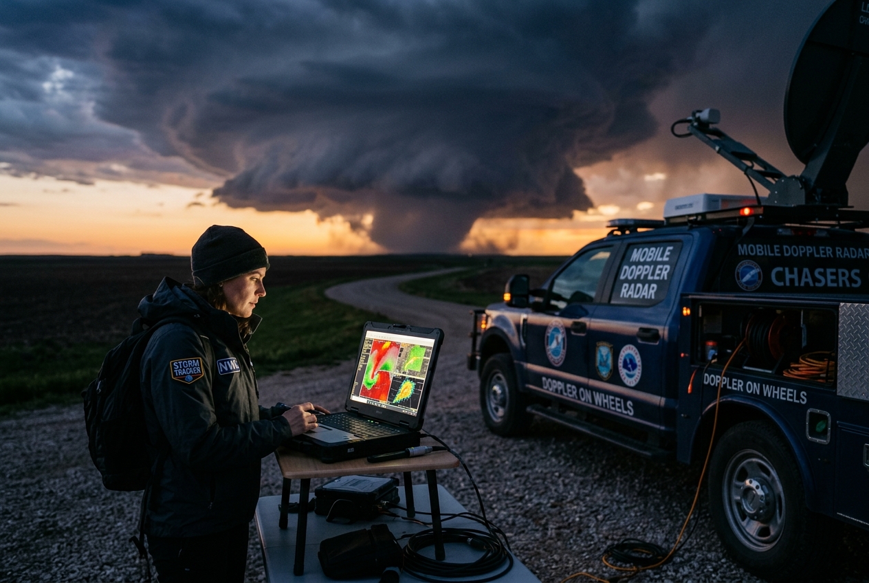
To an observer standing on the open plains of Oklahoma or the rolling terrain of the American Midwest, an impending severe convective storm communicates first through sensory immersion. Long before an S-band weather radar sweeps its target, the physical environment signals the thermodynamic engine at work. The air feels oppressive—thick with moisture, holding a dewpoint above $70^\circ\text{F}$ ($21^\circ\text{C}$). The wind at the surface, initially a weak southerly breeze, begins to back toward the southeast, drawing warm, moist maritime tropical air into the developing low-pressure center.
       TYPICAL DUAL-POLARIZATION RADAR BEAM PROFILES

 Horizontal Pulse (Z_H)           Vertical Pulse (Z_V)
 ───────────────────────►         ▲
                                  │
                                  │
 Raindrop (Oblate):               Raindrop (Oblate):
 Width > Height                   Width > Height
 High Reflectivity Backscatter    Moderate Reflectivity Backscatter

                 Z_DR = 10 * log10( Z_H / Z_V ) > 0 dB
Looking toward the horizon, the storm profile displays distinct structural hallmarks. A classic supercell presents a crisp, overshooting top penetrating the tropopause, flanked by a expansive anvil cloud spreading downwind along the jet stream. Beneath the dark storm base, a field observer notes the lowering known as the wall cloud—the visual manifestation of the storm's primary mesocyclone. A subtle color change often signals hidden danger: an eerie, bruised green tint across the precipitation core typically indicates heavy liquid water path content illuminated by sunlight scattering through high concentrations of large hail.
                  VISUAL & RADAR SUPERCELL ANATOMY

             Overshooting Top (Tropopause Penetration)
                       ▲
                       │     Anvil Cirrus Flow ──►
                ┌──────┴──────┐
                │             │
                │  UPDRAFT    │    Forward-Flank Downdraft (FFD)
                │   CORE      │   ┌───────────────────────────┐
                │             │   │ Rain & Hail Core          │
                └──────┬──────┘   │ High Z_H, Z_DR ~ 0 (Hail) │
                       │          └───────────────────────────┘
         Rear-Flank    │
       Downdraft (RFD) │ Wall Cloud / Mesocyclone
       ┌───────────────┴────────────────────────┐
       │ Clear Slot Notch   Tornado / TDS Zone  │
       │ Low Z_DR, Low rho_hv < 0.80            │
       └────────────────────────────────────────┘
As the rear-flank downdraft (RFD) cuts down on the back side of the wall cloud, a "clear slot" of sunshine or bright sky appears, dry air wrapping rapidly around the rotating column. The surface pressure drops sharply—often several millibars over tens of minutes—and the wind shifts violently, cooling by $10^\circ\text{C}$ to $15^\circ\text{C}$ within seconds as the cold pool arrives.
For the modern field meteorologist, linking these tactile atmospheric cues with real-time digital remote sensing is essential for accurate storm tracking and survival. Modern operational weather radar networks—such as the United States NOAA NEXRAD WSR-88D Network or the UK Met Office Weather Radar System—provide high-resolution volumetric scans every 2 to 5 minutes. Interpreting these scans requires mastering both classic Doppler velocity principles and advanced dual-polarization metrics.
2. Physical Principles & Intuitive Science: Dual-Polarization Metrics Demystified
Operational radar systems transmit pulses of microwave electromagnetic radiation—typically at S-band ($\sim 2.7 - 3.0\text{ GHz}$, wavelength $\lambda \approx 10\text{ cm}$) or C-band ($\sim 5.6\text{ GHz}$, wavelength $\lambda \approx 5\text{ cm}$). Legacy radar sent pulses with only horizontal linear polarization. Modern weather radar systems, however, utilize dual-polarization, simultaneously transmitting and receiving microwave energy polarized along both horizontal and vertical axes.
While conventional reflectivity ($Z$, measured in $\text{dBZ}$) measures the overall backscattered energy—which scales with the sixth power of drop diameter ($D^6$)—it suffers from severe ambiguity. A high reflectivity reading of $55\text{ dBZ}$ could signify torrential warm-rain downpours, a dense core of medium hail, or non-meteorological targets like swarms of insects or tornadic debris. Dual-polarization eliminates this ambiguity by examining three core variables: Differential Reflectivity ($Z_{DR}$), Specific Differential Phase ($K_{DP}$), and the Correlation Coefficient ($\rho_{hv}$).
┌────────────────────────────────────────────────────────────────────────────────────────┐
│                        DUAL-POLARIZATION METRIC MATRIX                                 │
├───────────────────────┬─────────────────────────┬──────────────────┬───────────────────┤
│ Target Type           │ Differential Ref. Z_DR  │ Spec. Diff Phase │ Corr. Coeff rho_hv│
│                       │ (dB)                    │ K_DP (deg/km)    │ (dimensionless)   │
├───────────────────────┼─────────────────────────┼──────────────────┼───────────────────┤
│ Small Raindrops       │ +0.2 to +1.0            │ 0.0 to 0.5       │ 0.98 to 1.00      │
│ Large Raindrops       │ +1.5 to +4.5            │ 1.0 to 6.0+      │ 0.97 to 0.99      │
│ Large Spherical Hail  │ -0.5 to +0.5            │ ~ 0.0            │ 0.93 to 0.97      │
│ Giant Tumbling Hail   │ -2.0 to -0.5            │ < 0.0 (bias)     │ 0.85 to 0.93      │
│ Tornadic Debris (TDS) │ -1.0 to +0.5            │ Near 0 / Erratic │ < 0.80 (often<0.6)│
│ Dry Snow / Ice Crystal│ 0.0 to +0.5             │ 0.0 to 0.2       │ 0.98 to 1.00      │
│ Melting Layer (Snow)  │ +1.0 to +3.0            │ 0.2 to 1.0       │ 0.85 to 0.94      │
└───────────────────────┴─────────────────────────┴──────────────────┴───────────────────┘
Differential Reflectivity ($Z_{DR}$)
Raindrops falling through the atmosphere are not rigid spheres; aerodynamic drag flattens them into oblate spheroids with flat bottoms, resembling hamburger buns. Larger drops experience greater flattening. Because their horizontal cross-section exceeds their vertical cross-section, their horizontal reflectivity ($Z_H$) is larger than their vertical reflectivity ($Z_V$).
Mathematically, Differential Reflectivity is expressed in decibels ($\text{dB}$):
$$Z_{DR} = 10 \log_{10} \left( \frac{Z_H}{Z_V} \right)$$
- $Z_{DR} > 0\text{ dB}$: Indicates horizontal oblate targets (e.g., medium to large raindrops).
- $Z_{DR} \approx 0\text{ dB}$: Indicates spherical targets (e.g., small drizzle drops or tumbling spherical hailstones).
- $Z_{DR} < 0\text{ dB}$: Indicates vertically oriented targets (e.g., ice crystals aligned by high-altitude electrical fields or tumbling conical hail falling point-first).
Specific Differential Phase ($K_{DP}$)
As an electromagnetic wave traverses a region of liquid precipitation, it slows down due to the higher dielectric constant of liquid water compared to air. Because oblate raindrops present a wider horizontal profile, the horizontally polarized wave experiences a greater phase shift than the vertically polarized wave. The accumulated phase difference is called the Differential Phase Shift ($\Phi_{DP}$).
The spatial derivative of $\Phi_{DP}$ along the radar beam path gives the Specific Differential Phase ($K_{DP}$), expressed in degrees per kilometer ($^\circ/\text{km}$):
$$K_{DP} = \frac{\Delta \Phi_{DP}}{2 \Delta r}$$
Where $\Delta r$ is the range increment. Unlike $Z$, which is dominated by giant hail ($D^6$), $K_{DP}$ is proportional to the total liquid water volume mass ($\sim D^3$) and is insensitive to dry hail or beam blockage. High $K_{DP}$ values ($> 2.0^\circ/\text{km}$) reliably locate extreme liquid rainfall rates, even when mixed with hail.
Correlation Coefficient ($\rho_{hv}$)
The Cross-Correlation Coefficient ($\rho_{hv}$) is a dimensionless statistical value between $0$ and $1$ measuring how uniformly the horizontal and vertical scatterers within a radar resolution volume behave in terms of shape, orientation, and phase structure.
$$\rho_{hv} = \frac{\sum (Z_H^{1/2} - \bar{Z}_H^{1/2})(Z_V^{1/2} - \bar{Z}_V^{1/2})}{\sqrt{\sum (Z_H - \bar{Z}_H) \sum (Z_V - \bar{Z}_V)}}$$
- $\rho_{hv} \ge 0.98$: Homogeneous meteorological targets (pure rain, uniform snow).
- $0.90 \le \rho_{hv} < 0.97$: Mixed-phase hydrometeors (melting snow, rain/hail mixtures).
- $\rho_{hv} < 0.80$: Highly irregular, non-meteorological scatterers (chaff, birds, insects, and lofted structural debris inside a tornado).
For authoritative reference on electromagnetic scattering in meteorological applications, consult the World Meteorological Organization Guide to Meteorological Instruments and the Wikipedia Dual-polarization Radar Entry.
3. Accessible Mathematical Foundations: Doppler Frequency Shifts & Rotational Shear Calculations
Part A: The Physics of the Doppler Frequency Shift
Every observer has experienced the classic acoustic Doppler effect: as an emergency vehicle approaches, its siren pitch sounds higher; as it drives away, the pitch drops. The radar antenna exploits this exact physical principle to calculate atmospheric wind velocities along the radar beam line of sight (radial velocity, $v_r$).
                 DOPPLER BEAM GEOMETRY & RADIAL VELOCITY

                  + v_r (Outbound / Motion away from radar)
                                ──────►
                  ┌───────────┐
      Radar       │ Target    │
     (Stationary) │ Air Parcel│
       ( ( ( ────►└───────────┘
                  ◄──────
                  - v_r (Inbound / Motion toward radar)
When a radar transmits an electromagnetic pulse of wavelength $\lambda$ at frequency $f_0$, the pulse strikes moving precipitation particles and reflects back to the antenna. The motion of the particles shifts the returned frequency by a small increment, known as the Doppler frequency shift ($f_d$).
The fundamental formula relating Doppler frequency shift to radial velocity is:
$$f_d = \frac{2 v_r}{\lambda}$$
Where:
* $f_d$ is the Doppler frequency shift (in Hertz, $\text{Hz}$ or $\text{s}^{-1}$).
* $v_r$ is the radial velocity of the target relative to the radar (in meters per second, $\text{m/s}$).
* $\lambda$ is the operational radar wavelength (in meters, $\text{m}$).
* The factor of $2$ accounts for the two-way path of the pulse (transmission to target and return to radar).
Real-World Worked Example: Doppler Frequency Calculation
Suppose an S-band radar operating at a wavelength $\lambda = 0.10\text{ m}$ ($10\text{ cm}$) measures a target moving directly toward the radar at a speed of $40\text{ m/s}$ (approximately $90\text{ mph}$). Calculate the resulting Doppler frequency shift.
Step 1: Identify the given quantities.
* $v_r = -40\text{ m/s}$ (inbound motion is conventionally negative).
* $\lambda = 0.10\text{ m}$.
Step 2: Substitute into the Doppler equation.
$$f_d = \frac{2 \times (-40\text{ m/s})}{0.10\text{ m}} = \frac{-80}{0.10} = -800\text{ Hz}$$
The radar's receiver signal processor detects a frequency shift of $-800\text{ Hz}$ relative to the carrier frequency $f_0$. By measuring this phase shift across successive pulses, the system determines that the air parcel is moving toward the dish at $40\text{ m/s}$.
Part B: Quantifying Rotational Shear Couplets in Severe Storms
On a velocity display (such as raw Radial Velocity or Storm-Relative Motion), the radar displays inbound velocities toward the antenna in cool colors (greens and blues) and outbound velocities away from the antenna in warm colors (reds and yellows).
When a rotating vortex (a mesocyclone or tornado) forms, inbound and outbound velocity maxima occur right next to each other at the same range and neighboring azimuths. This signature is called a velocity couplet or rotational shear couplet.
                   VELOCITY COUPLET SCHEMATIC (MESOCYCLONE)

                           Radar Beam Direction ──►

                     Azimuth Angle 1   Azimuth Angle 2
                   ┌─────────────────┬─────────────────┐
                   │                 │                 │
                   │  INBOUND PEAK   │  OUTBOUND PEAK  │
                   │  V_in = -35 m/s │  V_out = +45 m/s│
                   │  (Green/Blue)   │    (Red/Yellow) │
                   │                 │                 │
                   └─────────────────┴─────────────────┘
                   ◄───────────── D ──────────────────►
                              D = 2.5 km
To assess whether a mesocyclone is strong enough to trigger a Tornado Warning, meteorologists compute three critical metrics:
1. Rotational Velocity ($V_{rot}$): The average speed of the rotating winds.
2. Delta V ($\Delta V$): The total velocity differential across the couplet.
3. Azimuthal Shear ($S_{az}$): The spatial velocity change per unit distance across the core.
Governing Equations
$$\Delta V = |V_{in}| + |V_{out}|$$
$$V_{rot} = \frac{|V_{in}| + |V_{out}|}{2} = \frac{\Delta V}{2}$$
$$S_{az} = \frac{\Delta V}{D}$$
Where:
* $V_{in}$ is the peak inbound radial velocity magnitude ($\text{m/s}$).
* $V_{out}$ is the peak outbound radial velocity magnitude ($\text{m/s}$).
* $D$ is the linear distance between the inbound and outbound velocity peaks ($\text{m}$ or $\text{km}$).
Step-by-Step Numerical Example
A radar analyst observes a sharp velocity couplet embedded within a supercell wall cloud at a range of $45\text{ km}$. The radar data indicates:
* Peak inbound velocity: $V_{in} = -35\text{ m/s}$
* Peak outbound velocity: $V_{out} = +45\text{ m/s}$
* Distance between peaks across azimuths: $D = 2.5\text{ km} = 2,500\text{ m}$
Calculate $\Delta V$, $V_{rot}$, and the Azimuthal Shear ($S_{az}$).
Step 1: Compute Total Delta V ($\Delta V$).
$$\Delta V = |-35\text{ m/s}| + |45\text{ m/s}| = 35 + 45 = 80\text{ m/s}$$
Converting to knots: $80\text{ m/s} \times 1.94384 \approx 155.5\text{ knots}$.
Step 2: Compute Rotational Velocity ($V_{rot}$).
$$V_{rot} = \frac{80\text{ m/s}}{2} = 40\text{ m/s} \quad (\approx 77.8\text{ knots})$$
Step 3: Compute Azimuthal Shear ($S_{az}$).
$$S_{az} = \frac{\Delta V}{D} = \frac{80\text{ m/s}}{2500\text{ m}} = 0.032\text{ s}^{-1} = 3.2 \times 10^{-2}\text{ s}^{-1}$$
Diagnostic Significance
An azimuthal shear of $S_{az} \ge 0.02\text{ s}^{-1}$ ($20\text{ m/s per km}$) with $V_{rot} \ge 20\text{ m/s}$ ($40\text{ knots}$) meets standard operational thresholds for strong low-level mesocyclonic rotation. An $S_{az} = 0.032\text{ s}^{-1}$ represents intense rotational shear, strongly indicative of impending or ongoing tornadogenesis. For background on operational thresholds, see NOAA's National Weather Service JetStream Doppler Guide.
4. Real-World Observational Techniques: Signature Breakdown & Field Fingerprints
Combining reflectivity, Doppler velocity, and dual-polarization metrics enables unambiguous identification of critical severe weather processes in real-time.
                  DUAL-POLARIZATION SIGNATURE IDENTIFICATION

     HAIL CORE                     TORNADIC DEBRIS (TDS)         MELTING LAYER (BRIGHT BAND)
 ┌───────────────────────────┐  ┌───────────────────────────┐  ┌───────────────────────────┐
 │ Z_H:   > 60 dBZ (Very High)│  │ Z_H:   > 45-50 dBZ (High) │  │ Z_H:   35 - 50 dBZ (Moderate)│
 │ Z_DR:  -0.5 to +0.5 dB    │  │ Z_DR:  -1.5 to +0.5 dB    │  │ Z_DR:  +1.5 to +3.5 dB    │
 │ K_DP:  Low (dry) / High   │  │ K_DP:  Erratic / Near 0   │  │ K_DP:  0.2 to 0.8 deg/km  │
 │ rho_hv:0.88 - 0.94        │  │ rho_hv: < 0.80 (Sharp Drop)│ │ rho_hv: 0.85 - 0.93       │
 └───────────────────────────┘  └───────────────────────────┘  └───────────────────────────┘
1. Differentiating Hail Cores & $Z_{DR}$ Columns
Large hailstones tumble randomly as they fall. Because their orientation is unbiased, their average horizontal and vertical dimensions are equivalent ($Z_H \approx Z_V$). Consequently, a massive hail core exhibits:
* Extremely High Reflectivity ($Z_H > 60 - 70\text{ dBZ}$).
* Near-Zero Differential Reflectivity ($Z_{DR} \approx -0.5\text{ to } +0.5\text{ dB}$).
       HAIL CORE VS. RAIN SHIELD RADAR PROFILE

 Reflectivity (Z_H)           Differential Reflectivity (Z_DR)
 ┌─────────────────────────┐  ┌─────────────────────────┐
 │ Rain:  35 - 45 dBZ      │  │ Rain:  +1.5 to +3.5 dB  │
 │ Hail:  60 - 70+ dBZ     │  │ Hail:  -0.5 to +0.5 dB  │
 └─────────────────────────┘  └─────────────────────────┘
$Z_{DR}$ Columns
Updrafts carry liquid water drops above the environmental freezing level ($0^\circ\text{C}$ isosurface) before they can freeze into graupel or hail. Supercooled raindrops floating upward inside the core produce a vertical plume of elevated $Z_{DR}$ ($+2.0\text{ to } +4.0\text{ dB}$) extending several kilometers above the freezing level. This $Z_{DR}$ column identifies the core of a powerful thunderstorm updraft. Tracking the height and growth rate of a $Z_{DR}$ column gives meteorologists direct warning of hail growth before hailstones reach the ground.
2. Identifying Tornadic Debris Signatures (TDS)
Prior to dual-polarization technology, determining whether a velocity couplet was actively producing a ground-contact tornado relied entirely on spotter reports. Dual-polarization radar solved this by detecting lofted debris (branches, sheet metal, insulation, soil).
A confirmed Tornadic Debris Signature (TDS)—often colloquially termed a "debris ball"—requires three co-located criteria:
1. Strong Low-Level Rotational Velocity Couplet ($V_{rot} \ge 20 - 25\text{ m/s}$).
2. Elevated Reflectivity Core ($Z_H \ge 45 - 50\text{ dBZ}$) co-located with the rotation center.
3. Sharp Drop in Correlation Coefficient ($\rho_{hv} < 0.80$, often dropping below $0.55$).
Because lofted structural debris consists of highly irregular, chaotic shapes tumbling in mid-air, the radar's horizontal and vertical returns become completely uncorrelated, resulting in a dramatic drop in $\rho_{hv}$. Detecting a TDS confirming ground damage allows forecasters to issue high-priority Tornado Warnings with exceptional confidence.
                   TORNADIC DEBRIS SIGNATURE (TDS) PROFILE

  Co-located Radar Products at Vortex Center:

   Storm Relative Motion        Reflectivity (Z_H)           Corr. Coeff (rho_hv)
  ┌─────────────────────────┐  ┌─────────────────────────┐  ┌─────────────────────────┐
  │ Strong Couplet          │  │ High Core               │  │ Sharp Crash             │
  │ V_rot = 35 m/s          │  │ Z_H = 52 dBZ            │  │ rho_hv = 0.58           │
  │ (Green / Red Touch)     │  │ (Debris Ball)           │  │ (Lofted Debris)         │
  └─────────────────────────┘  └─────────────────────────┘  └─────────────────────────┘
3. Locating Rain-Snow Boundaries & The Melting Layer ("Bright Band")
In stratiform precipitation systems or winter winter storms, radar beams intercepting the altitude where ice crystals melt into liquid rain encounter the melting layer, visually recognized on legacy radar displays as a band of enhanced reflectivity called the Bright Band.
As snowflakes descend through the $0^\circ\text{C}$ isotherm:
1. Snowflakes begin to melt, forming a coating of liquid water over their large, irregular ice structures.
2. Because liquid water has a dielectric factor nearly 5 times higher than ice, the radar perceives these water-coated giant aggregates as enormous raindrops, causing reflectivity to jump artificially ($Z_H \sim 40-50\text{ dBZ}$).
3. As snowflakes melt completely, they collapse into smaller, rapidly falling raindrops, causing reflectivity to drop below the melting layer.
Dual-Polarization Fingerprint of the Melting Layer:
- Reflectivity ($Z_H$): Locally elevated ($+5\text{ to } +10\text{ dBZ}$ boost in the melting strip).
- Differential Reflectivity ($Z_{DR}$): High ($+1.5\text{ to } +3.5\text{ dB}$), caused by melting snow aggregates flattening horizontally as they fall.
- Correlation Coefficient ($\rho_{hv}$): Characteristic ring or stripe of lowered values ($\rho_{hv} \approx 0.86 - 0.94$), reflecting the chaotic mixture of water, wet snow, and dry snow.
               VERTICAL ATMOSPHERIC RADAR MELTING CROSS-SECTION

 Altitude (km)  Phase State          Z_H      Z_DR        rho_hv
 ──────────────────────────────────────────────────────────────────
  4.0 km        Dry Snow / Ice       20 dBZ   +0.2 dB     0.99
  3.0 km        Melting Aggregates   45 dBZ   +2.5 dB     0.88  ◄── Bright Band
  1.5 km        Pure Liquid Rain     32 dBZ   +1.1 dB     0.99
For further research into snow-rain transition physics, access reference material at MIT OpenCourseWare Radar Meteorology.
5. Practical Weather Forecasting & Outdoor Guidance: Translating Radar Screens to Life-Saving Field Decisions
For storm chasers, emergency responders, and outdoor enthusiasts, interpreting radar data accurately requires recognizing physical radar limitations while following systematic diagnostic steps.
              REAL-TIME SEVERE WEATHER DECISION FLOWCHART

                      [ Inspect Base Reflectivity (Z_H) ]
                                      │
                         Is Z_H > 50 dBZ in storm core?
                        ┌─────────────┴─────────────┐
                       YES                         NO
                        │                           │
              [ Check Z_DR Metric ]       [ Track System Motion & ]
             ┌──────────┴──────────┐      [ Monitor Stratiform    ]
          Z_DR ~ 0 dB         Z_DR > 2 dB [ Rain Boundaries       ]
             │                     │
      (Hail Risk Core)     (Heavy Rain Core)
             │                     │
  [ Inspect Velocity ]     [ Inspect K_DP ]
  [ Couplet Shear    ]     [ Flash Flood Risk ]
             │
     Couplet Present?
    ┌────────┴────────┐
   YES               NO
    │                 │
[ Check rho_hv ]  [ Severe Wind / ]
[ for TDS Drop ]  [ Hail Threat   ]
    │
 rho_hv < 0.80?
  ┌─┴─┐
 YES  NO
  │   │
 (CONFIRMED TORNADO / DEBRIS LOFTED) ──► ISSUE IMMEDIATE EMERGENCY SHELTER ACTION
Common Radar Artifacts and Mitigations
- Velocity Aliasing (Nyquist Limit): When actual radial wind speeds exceed the maximum unambiguous velocity interval ($v_{max} = \frac{\lambda \cdot PRF}{4}$, where $PRF$ is Pulse Repetition Frequency), the radar receiver folds the velocity values. An extreme inbound velocity of $-45\text{ m/s}$ may suddenly appear as a false outbound $+15\text{ m/s}$. Modern radar algorithms automatically de-alias velocity fields, but raw data displays can occasionally present false couplets along aliasing boundaries.
- Three-Body Scatter Spike (TBSS): A linear spike of low reflectivity and low $\rho_{hv}$ extending directly down-range along the radar beam behind an intense hail core. The spike is caused by microwave radiation bouncing from the radar to large hailstones, scattering down to the ground, reflecting back up to the hailstones, and finally returning to the radar dish. A TBSS is a definitive indicator of large, damaging hail ($D > 2.5\text{ cm} / 1\text{ inch}$).
6. Takeaway Box: Today's Meteorological Rule of Thumb
[!IMPORTANT]
Today's Meteorological Rule of Thumb: The Severe Storm Dual-Pol Triad
When evaluating a severe convective storm cell on dual-polarization radar, remember the three cardinal diagnostic signatures:
- The Hail Identification Rule: If Reflectivity ($Z_H$) exceeds $60\text{ dBZ}$ while Differential Reflectivity ($Z_{DR}$) drops toward $0.0\text{ dB}$, you are looking at a dense falling hail core, not giant raindrops. If $Z_{DR}$ drops below zero ($-1.0\text{ dB}$), massive tumbling hailstones are present.
- The Tornado Debris Signature (TDS) Rule: A rotational velocity couplet with an Azimuthal Shear $S_{az} \ge 0.02\text{ s}^{-1}$ is a mesocyclone. If the Correlation Coefficient ($\rho_{hv}$) simultaneously drops below $0.80$ directly over the vortex core, a tornado is actively destroying ground structures and lofting debris into the air.
- The Flash Flood ($K_{DP}$) Rule: Never rely on reflectivity alone to estimate heavy rainfall in hail storms. Look for $K_{DP} > 2.0^\circ/\text{km}$. $K_{DP}$ responds exclusively to liquid water mass, providing an accurate measure of torrential precipitation rates regardless of mixed hail.
Summary Checklist for Field Observers
- Step 1: Monitor surface temperature, dewpoint, and wind direction for back-building inflow patterns.
- Step 2: Locate storm updrafts using vertical $Z_{DR}$ columns extending above the $0^\circ\text{C}$ isotherm.
- Step 3: Calculate rotational velocity ($V_{rot}$) and azimuthal shear ($S_{az}$) across velocity couplets to quantify tornado potential.
- Step 4: Confirm ground impact by cross-referencing low-level velocity couplets with sharp localized crashes in $\rho_{hv}$.
External References & Further Reading
- NOAA National Severe Storms Laboratory (NSSL) Dual-Pol Radar Research
- National Weather Service JetStream: Doppler Radar & Velocity Principles
- UK Met Office Operational Weather Radar Network Technical Overview
- World Meteorological Organization (WMO) Meteorological Instruments & Methods Guide
- Wikipedia Entry on Weather Radar and Dual-Polarization Metrics
- MIT OpenCourseWare: Atmospheric Remote Sensing & Radar Meteorology