Quantum Entanglement: Quantifying Non-Local Correlations and Bell State Operations in Composite Qubit Systems
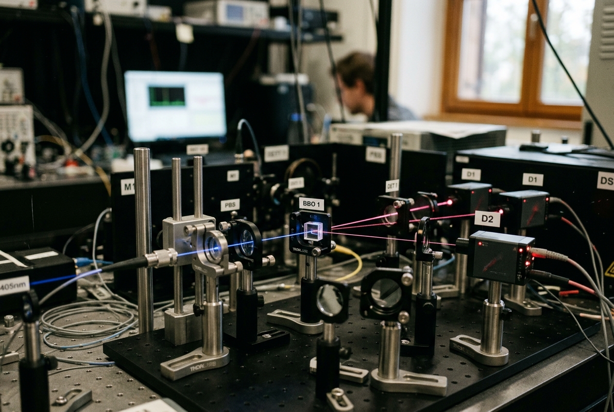
An academically rigorous analysis of composite Hilbert spaces, maximally entangled Bell states, CHSH inequality proofs, and operational protocols driving the second quantum revolution.
1. Theoretical Foundations: Kinematics of Composite Quantum Systems
Quantum mechanics departs fundamentally from classical physics in its description of composite systems. Where classical state spaces combine via the Cartesian product—scaling linearly with component additions ($\mathbb{R}^{d_A \times d_B} = \mathbb{R}^{d_A} \times \mathbb{R}^{d_B}$)—quantum mechanics requires the algebraic tensor product of Hilbert spaces. This structural rule lies at the heart of quantum non-locality, quantum information processing, and the exponential expansion of quantum state space.
Single Qubit Kinematics and Bloch Sphere Geometry
A single quantum bit (qubit) is defined in a two-dimensional complex Hilbert space $\mathcal{H}_2 \cong \mathbb{C}^2$. The canonical computational basis vectors, denoted in Dirac bra-ket notation, are:
$$|0\rangle = \begin{pmatrix} 1 \ 0 \end{pmatrix}, \quad |1\rangle = \begin{pmatrix} 0 \ 1 \end{pmatrix}$$
An arbitrary pure single-qubit state $|\psi\rangle \in \mathcal{H}_2$ is represented as a normalized linear superposition:
$$|\psi\rangle = \alpha |0\rangle + \beta |1\rangle, \quad \text{where } \alpha, \beta \in \mathbb{C} \quad \text{and} \quad |\alpha|^2 + |\beta|^2 = 1$$
Because global complex phase factors $e^{i\gamma}$ yield identical measurement statistics, a single-qubit state vector can be uniquely mapped onto the three-dimensional unit sphere $\mathbb{S}^2 \subset \mathbb{R}^3$, known as the Bloch sphere. Parameterizing the complex coefficients using spherical coordinates yields:
$$|\psi(\theta, \phi)\rangle = \cos\left(\frac{\theta}{2}\right) |0\rangle + e^{i\phi} \sin\left(\frac{\theta}{2}\right) |1\rangle$$
where $\theta \in [0, \pi]$ denotes the polar angle (governing relative populations of $|0\rangle$ and $|1\rangle$) and $\phi \in [0, 2\pi)$ represents the azimuthal angle (governing quantum relative phase).
                  |0>  (North Pole, θ = 0)
                   |
                   |   /
                   |  /  |ψ⟩ = cos(θ/2)|0⟩ + e^(iφ)sin(θ/2)|1⟩
                   | /
                   |/____ (Equator, θ = π/2)
                  / \
                 /   \
                /     \
               /       |1>  (South Pole, θ = π)
The density matrix $\rho$ representing a pure single-qubit state is given by the outer product $\rho = |\psi\rangle\langle\psi|$. In terms of the vector of Pauli matrices $\boldsymbol{\sigma} = (\sigma_x, \sigma_y, \sigma_z)$, any valid density matrix (pure or mixed) can be expanded as:
$$\rho = \frac{1}{2}\left( I + \mathbf{r} \cdot \boldsymbol{\sigma} \right) = \frac{1}{2}\left( I + r_x \sigma_x + r_y \sigma_y + r_z \sigma_z \right)$$
where $\mathbf{r} = (r_x, r_y, r_z) \in \mathbb{R}^3$ is the Bloch vector. Pure states lie strictly on the surface ($||\mathbf{r}||_2 = 1$), whereas mixed states satisfy $||\mathbf{r}||_2 < 1$, with the maximally mixed state located at the origin ($\mathbf{r} = \mathbf{0}$, $\rho = \frac{1}{2}I$).
The Tensor Product Structure of Composite Hilbert Spaces
When combining two distinct quantum subsystems $A$ and $B$, governed by Hilbert spaces $\mathcal{H}_A$ and $\mathcal{H}_B$ of dimensions $d_A$ and $d_B$, the composite system's state space is the tensor product Hilbert space:
$$\mathcal{H}_{AB} = \mathcal{H}_A \otimes \mathcal{H}_B$$
The dimension of $\mathcal{H}{AB}$ is $d{AB} = d_A \times d_B$. For an $n$-qubit system, the Hilbert space is $\mathcal{H}_{2^n} = (\mathbb{C}^2)^{\otimes n}$, possessing dimension $2^n$. This exponential expansion of basis states forms the mathematical bedrock of quantum computational speedup, as explored in authoritative literature such as Wikipedia's Quantum Entanglement Overview.
Let ${|i\rangle_A}{i=0}^{d_A-1}$ and ${|j\rangle_B}{j=0}^{d_B-1}$ be orthonormal bases for $\mathcal{H}A$ and $\mathcal{H}_B$. The canonical basis for $\mathcal{H}{AB}$ comprises the tensor products:
$$|i\rangle_A \otimes |j\rangle_B \equiv |i\rangle |j\rangle \equiv |ij\rangle_{AB}$$
For a two-qubit system ($d_A = d_B = 2$), the computational basis consists of four 4-dimensional vectors:
$$|00\rangle = \begin{pmatrix} 1 \ 0 \ 0 \ 0 \end{pmatrix}, \quad |01\rangle = \begin{pmatrix} 0 \ 1 \ 0 \ 0 \end{pmatrix}, \quad |10\rangle = \begin{pmatrix} 0 \ 0 \ 1 \ 0 \end{pmatrix}, \quad |11\rangle = \begin{pmatrix} 0 \ 0 \ 0 \ 1 \end{pmatrix}$$
An arbitrary two-qubit pure state $|\Psi\rangle_{AB} \in \mathcal{H}_{AB}$ is expressed as:
$$|\Psi\rangle_{AB} = \sum_{i=0}^{1} \sum_{j=0}^{1} c_{ij} |ij\rangle = c_{00}|00\rangle + c_{01}|01\rangle + c_{10}|10\rangle + c_{11}|11\rangle$$
where $c_{ij} \in \mathbb{C}$ and the normalization condition dictates $\sum_{i,j} |c_{ij}|^2 = 1$.
Classical Composition (Cartesian):    Dim(A × B) = Dim(A) + Dim(B)  ==> Linear scaling
Quantum Composition (Tensor Product): Dim(A ⊗ B) = Dim(A) × Dim(B)  ==> Exponential scaling (2ⁿ)
Product States vs. Entangled States
A state $|\Psi\rangle_{AB} \in \mathcal{H}_{AB}$ is classified as a product state (or factorizable state) if and only if there exist individual subsystem state vectors $|\phi\rangle_A \in \mathcal{H}_A$ and $|\chi\rangle_B \in \mathcal{H}_B$ such that:
$$|\Psi\rangle_{AB} = |\phi\rangle_A \otimes |\chi\rangle_B$$
If no such factorization exists, the state is defined as entangled. Physical measurement of subsystem $A$ in a product state leaves the state of subsystem $B$ completely invariant. Conversely, in an entangled state, subsystems do not possess individual state vectors; their physical properties are fundamentally non-separable.
Formal Criterion via Schmidt Decomposition
Any pure bipartite state $|\Psi\rangle_{AB} \in \mathcal{H}_A \otimes \mathcal{H}_B$ can be written in its Schmidt decomposition:
$$|\Psi\rangle_{AB} = \sum_{k=1}^{r} \lambda_k |u_k\rangle_A \otimes |v_k\rangle_B$$
where $\lambda_k > 0$ are real positive scalars called Schmidt coefficients satisfying $\sum_{k=1}^r \lambda_k^2 = 1$, ${|u_k\rangle_A}$ and ${|v_k\rangle_B}$ are orthonormal sets in $\mathcal{H}A$ and $\mathcal{H}_B$, and $r \le \min(d_A, d_B)$ is the Schmidt rank of $|\Psi\rangle{AB}$.
- Product State Criterion: Schmidt rank $r = 1$.
- Entangled State Criterion: Schmidt rank $r > 1$.
Quantitative Entanglement via Partial Trace and Purity
To evaluate the physical state of subsystem $A$ alone, we construct the reduced density matrix $\rho_A$ by performing a partial trace over subsystem $B$:
$$\rho_A = \text{Tr}B(\rho{AB}) = \text{Tr}B(|\Psi\rangle{AB}\langle\Psi|)$$
Given the Schmidt decomposition of $|\Psi\rangle_{AB}$, the reduced density matrix simplifies to:
$$\rho_A = \text{Tr}B \left( \sum{k,l} \lambda_k \lambda_l |u_k\rangle_A\langle u_l| \otimes |v_k\rangle_B\langle v_l| \right) = \sum_{k=1}^{r} \lambda_k^2 |u_k\rangle_A\langle u_k|$$
The purity $\gamma(\rho_A) = \text{Tr}(\rho_A^2)$ provides an absolute metric of entanglement:
$$\gamma(\rho_A) = \sum_{k=1}^r \lambda_k^4$$
- For a product state ($r=1, \lambda_1=1$), $\rho_A = |u_1\rangle_A\langle u_1|$ is a pure state with purity $\gamma(\rho_A) = 1$.
- For a maximally entangled state of two qubits ($r=2, \lambda_1=\lambda_2=\frac{1}{\sqrt{2}}$), the reduced density matrix is maximally mixed:
$$\rho_A = \frac{1}{2}|u_1\rangle_A\langle u_1| + \frac{1}{2}|u_2\rangle_A\langle u_2| = \frac{1}{2}I_A$$
with purity $\gamma(\rho_A) = \frac{1}{2}$ and von Neumann entropy $S(\rho_A) = -\text{Tr}(\rho_A \log_2 \rho_A) = 1\text{ bit}$. This reflects a profound quantum paradox: while complete physical information is known about the bipartite system as a whole ($S(\rho_{AB}) = 0$), zero physical information is contained within either individual subsystem ($S(\rho_A) = 1$).
2. Derivation and Canonical Algebra of the Four Bell States
The canonical maximally entangled states of two qubits are known as the Bell states or EPR pairs. They form an orthonormal basis for $\mathcal{H}_4 = \mathbb{C}^2 \otimes \mathbb{C}^2$, termed the Bell basis.
                   +---+      +---+
    |0⟩_A ---------| H |------| • |------- (|00⟩ + |11⟩) / √2  =  |Φ+⟩
                   +---+      |   |
                             | X |
    |0⟩_B -------------------|   |-------
                              +---+
                                CNOT
Quantum Circuit Construction
The standard quantum circuit generating the Bell state $|\Phi^+\rangle_{AB}$ operates on unentangled initial register $|0\rangle_A \otimes |0\rangle_B$. The sequence applies a Hadamard gate ($H$) to qubit $A$, followed by a Controlled-NOT ($CX$) gate with qubit $A$ as control and qubit $B$ as target.
Step-by-Step Operator Algebra
- Initial Unentangled State:
$$|\psi_0\rangle = |0\rangle_A |0\rangle_B = \begin{pmatrix} 1 \ 0 \ 0 \ 0 \end{pmatrix}$$
- Application of Hadamard Gate to Qubit A:
The composite operator is $H \otimes I_2$. The Hadamard matrix is $H = \frac{1}{\sqrt{2}}\begin{pmatrix} 1 & 1 \ 1 & -1 \end{pmatrix}$.
$$|\psi_1\rangle = (H \otimes I_2)|00\rangle = \left( \frac{|0\rangle_A + |1\rangle_A}{\sqrt{2}} \right) \otimes |0\rangle_B = \frac{1}{\sqrt{2}}|00\rangle + \frac{1}{\sqrt{2}}|10\rangle$$
In matrix form:
$$|\psi_1\rangle = \frac{1}{\sqrt{2}} \begin{pmatrix} 1 & 0 & 1 & 0 \ 0 & 1 & 0 & 1 \ 1 & 0 & -1 & 0 \ 0 & 1 & 0 & -1 \end{pmatrix} \begin{pmatrix} 1 \ 0 \ 0 \ 0 \end{pmatrix} = \frac{1}{\sqrt{2}} \begin{pmatrix} 1 \ 0 \ 1 \ 0 \end{pmatrix}$$
- Application of Controlled-NOT (CNOT) Gate:
The CNOT matrix in the standard basis ${|00\rangle, |01\rangle, |10\rangle, |11\rangle}$ is:
$$CX = \begin{pmatrix} 1 & 0 & 0 & 0 \ 0 & 1 & 0 & 0 \ 0 & 0 & 0 & 1 \ 0 & 0 & 1 & 0 \end{pmatrix}$$
Applying $CX$ to $|\psi_1\rangle$:
$$|\psi_2\rangle = CX |\psi_1\rangle = \frac{1}{\sqrt{2}} \begin{pmatrix} 1 & 0 & 0 & 0 \ 0 & 1 & 0 & 0 \ 0 & 0 & 0 & 1 \ 0 & 0 & 1 & 0 \end{pmatrix} \begin{pmatrix} 1 \ 0 \ 1 \ 0 \end{pmatrix} = \frac{1}{\sqrt{2}} \begin{pmatrix} 1 \ 0 \ 0 \ 1 \end{pmatrix} = \frac{|00\rangle + |11\rangle}{\sqrt{2}} \equiv |\Phi^+\rangle$$
The Bell State Family
By varying the initial basis inputs $|a\rangle_A |b\rangle_B \in {|00\rangle, |01\rangle, |10\rangle, |11\rangle}$, or by applying single-qubit Pauli operations $(\sigma_x, \sigma_y, \sigma_z)$ locally to qubit $A$ of $|\Phi^+\rangle$, we span the complete set of four Bell states:
$$\begin{aligned}
|\Phi^+\rangle &= \frac{1}{\sqrt{2}}(|00\rangle + |11\rangle) = (I \otimes I)|\Phi^+\rangle \
|\Phi^-\rangle &= \frac{1}{\sqrt{2}}(|00\rangle - |11\rangle) = (\sigma_z \otimes I)|\Phi^+\rangle \
|\Psi^+\rangle &= \frac{1}{\sqrt{2}}(|01\rangle + |10\rangle) = (\sigma_x \otimes I)|\Phi^+\rangle \
|\Psi^-\rangle &= \frac{1}{\sqrt{2}}(|01\rangle - |10\rangle) = (-i\sigma_y \otimes I)|\Phi^+\rangle
\end{aligned}$$
Matrix Representations and Completeness
Written as 4D column vectors:
$$|\Phi^+\rangle = \frac{1}{\sqrt{2}}\begin{pmatrix} 1 \ 0 \ 0 \ 1 \end{pmatrix}, \quad |\Phi^-\rangle = \frac{1}{\sqrt{2}}\begin{pmatrix} 1 \ 0 \ 0 \ -1 \end{pmatrix}, \quad |\Psi^+\rangle = \frac{1}{\sqrt{2}}\begin{pmatrix} 0 \ 1 \ 1 \ 0 \end{pmatrix}, \quad |\Psi^-\rangle = \frac{1}{\sqrt{2}}\begin{pmatrix} 0 \ 1 \ -1 \ 0 \end{pmatrix}$$
These states satisfy orthonormality:
$$\langle B_i | B_j \rangle = \delta_{ij} \quad \text{for } |B_i\rangle, |B_j\rangle \in {|\Phi^+\rangle, |\Phi^-\rangle, |\Psi^+\rangle, |\Psi^-\rangle}$$
and completeness over the 4-dimensional composite space:
$$\sum_{i=1}^4 |B_i\rangle\langle B_i| = I_4$$
3. Local Realism, Hidden Variables, and the Mathematical Proof of the CHSH Inequality
In 1935, Albert Einstein, Boris Podolsky, and Nathan Rosen (EPR) published their foundational critique asserting that quantum mechanics was incomplete. They argued that if physical measurements performed on spatially separated systems yield correlated outcomes without disturbing one another, there must exist underlying elements of reality—local hidden variables—that deterministically govern measurement results prior to observation.
Detailed computational and philosophical analyses of Bell's theorem can be found at the Stanford Encyclopedia of Philosophy: Bell's Theorem.
                 EPR / Local Realism Premise:
           λ (Hidden Variable set at source)
                     /         \
                    /           \
                   v             v
            Alice Measurement  Bob Measurement
            A(a, λ) ∈ {-1, +1}  B(b, λ) ∈ {-1, +1}
Formalization of Local Hidden Variable (LHV) Theories
Consider a source emitting pairs of qubits to two distant observers, Alice and Bob. Alice chooses to measure observable $A$ parameterized by detector angle vector $\mathbf{a}$, yielding outcome $A(\mathbf{a}) \in {-1, +1}$. Bob measures observable $B$ parameterized by angle vector $\mathbf{b}$, yielding outcome $B(\mathbf{b}) \in {-1, +1}$.
A Local Hidden Variable (LHV) model postulates:
1. Realism: The measurement outcomes are determined by a set of hidden parameters $\lambda \in \Lambda$ distributed according to a probability distribution $p(\lambda)$ such that $\int_\Lambda p(\lambda) d\lambda = 1$.
2. Locality: Alice's outcome depends exclusively on her setting $\mathbf{a}$ and $\lambda$, remaining independent of Bob's choice $\mathbf{b}$ or outcome $B$. Similarly, Bob's outcome depends exclusively on $\mathbf{b}$ and $\lambda$.
Thus, the joint expectation value of observables $A(\mathbf{a})$ and $B(\mathbf{b})$ under LHV is written:
$$E(\mathbf{a}, \mathbf{b}) = \int_{\Lambda} A(\mathbf{a}, \lambda) B(\mathbf{b}, \lambda) p(\lambda) d\lambda$$
where $A(\mathbf{a}, \lambda) = \pm 1$ and $B(\mathbf{b}, \lambda) = \pm 1$.
Derivation of the CHSH Inequality
The Clauser-Horne-Shimony-Holt (CHSH) formulation considers two alternate detector settings for Alice ($\mathbf{a}, \mathbf{a}'$) and two for Bob ($\mathbf{b}, \mathbf{b}'$). Define the CHSH correlation random variable $C(\lambda)$ for a given hidden state $\lambda$:
$$C(\lambda) = A(\mathbf{a}, \lambda)B(\mathbf{b}, \lambda) - A(\mathbf{a}, \lambda)B(\mathbf{b}', \lambda) + A(\mathbf{a}', \lambda)B(\mathbf{b}, \lambda) + A(\mathbf{a}', \lambda)B(\mathbf{b}', \lambda)$$
Factorizing the expression:
$$C(\lambda) = A(\mathbf{a}, \lambda) \left[ B(\mathbf{b}, \lambda) - B(\mathbf{b}', \lambda) \right] + A(\mathbf{a}', \lambda) \left[ B(\mathbf{b}, \lambda) + B(\mathbf{b}', \lambda) \right]$$
Since $B(\mathbf{b}, \lambda), B(\mathbf{b}', \lambda) \in {-1, +1}$, one of the bracketed terms must equal zero while the other must equal $\pm 2$:
* If $B(\mathbf{b}, \lambda) = B(\mathbf{b}', \lambda)$, then $B(\mathbf{b}, \lambda) - B(\mathbf{b}', \lambda) = 0$ and $B(\mathbf{b}, \lambda) + B(\mathbf{b}', \lambda) = \pm 2$.
* If $B(\mathbf{b}, \lambda) \neq B(\mathbf{b}', \lambda)$, then $B(\mathbf{b}, \lambda) - B(\mathbf{b}', \lambda) = \pm 2$ and $B(\mathbf{b}, \lambda) + B(\mathbf{b}', \lambda) = 0$.
Since $|A(\mathbf{a}, \lambda)| = 1$ and $|A(\mathbf{a}', \lambda)| = 1$, it follows strictly that for every individual realization $\lambda$:
$$|C(\lambda)| = 2$$
Integrating over the distribution space $\Lambda$:
$$\begin{aligned}
|S_{\text{classical}}| &= \left| \int_{\Lambda} C(\lambda) p(\lambda) d\lambda \right| \le \int_{\Lambda} |C(\lambda)| p(\lambda) d\lambda \
&\le \int_{\Lambda} 2 \, p(\lambda) d\lambda = 2 \int_{\Lambda} p(\lambda) d\lambda = 2
\end{aligned}$$
Thus, we obtain the Classical CHSH Inequality:
$$S_{\text{CHSH}} = |E(\mathbf{a}, \mathbf{b}) - E(\mathbf{a}, \mathbf{b}') + E(\mathbf{a}', \mathbf{b}) + E(\mathbf{a}', \mathbf{b}')| \le 2$$
Quantum Mechanical Violation and Tsirelson's Bound
Now we evaluate the quantum mechanical expectation value $E_{\text{QM}}(\mathbf{a}, \mathbf{b}) = \langle \Phi^+ | (\mathbf{a} \cdot \boldsymbol{\sigma}) \otimes (\mathbf{b} \cdot \boldsymbol{\sigma}) | \Phi^+ \rangle$.
Let the single-qubit spin projection observables in the $x-z$ plane be:
$$\mathbf{a} \cdot \boldsymbol{\sigma} = \sin\theta_a \sigma_x + \cos\theta_a \sigma_z, \quad \mathbf{b} \cdot \boldsymbol{\sigma} = \sin\theta_b \sigma_x + \cos\theta_b \sigma_z$$
For the Bell state $|\Phi^+\rangle = \frac{1}{\sqrt{2}}(|00\rangle + |11\rangle)$, direct calculation yields:
$$E_{\text{QM}}(\mathbf{a}, \mathbf{b}) = \mathbf{a} \cdot \mathbf{b} = \cos(\theta_a - \theta_b)$$
To maximize the CHSH expression, select coplanar measurement angles in the $x-z$ plane:
$$\theta_a = 0, \quad \theta_{a'} = \frac{\pi}{2}, \quad \theta_b = \frac{\pi}{4}, \quad \theta_{b'} = -\frac{\pi}{4}$$
Calculating individual expectation values:
$$\begin{aligned}
E(\mathbf{a}, \mathbf{b}) &= \cos\left(0 - \frac{\pi}{4}\right) = \cos\left(-\frac{\pi}{4}\right) = \frac{\sqrt{2}}{2} \
E(\mathbf{a}, \mathbf{b}') &= \cos\left(0 - \left(-\frac{\pi}{4}\right)\right) = \cos\left(\frac{\pi}{4}\right) = \frac{\sqrt{2}}{2} \
E(\mathbf{a}', \mathbf{b}) &= \cos\left(\frac{\pi}{2} - \frac{\pi}{4}\right) = \cos\left(\frac{\pi}{4}\right) = \frac{\sqrt{2}}{2} \
E(\mathbf{a}', \mathbf{b}') &= \cos\left(\frac{\pi}{2} - \left(-\frac{\pi}{4}\right)\right) = \cos\left(\frac{3\pi}{4}\right) = -\frac{\sqrt{2}}{2}
\end{aligned}$$
Substituting into the CHSH parameter $S$:
$$S_{\text{QM}} = \left| \frac{\sqrt{2}}{2} - \left(-\frac{\sqrt{2}}{2}\right) + \frac{\sqrt{2}}{2} + \frac{\sqrt{2}}{2} \right| = \left| 4 \cdot \frac{\sqrt{2}}{2} \right| = 2\sqrt{2} \approx 2.8284$$
CHSH Bound Spectrum:
|-----------------------|-----------------------|
0                       2 (LHV Limit)         2√2 ≈ 2.828 (Tsirelson Bound / Quantum Limit)
The value $S_{\text{QM}} = 2\sqrt{2}$ exceeds the local realistic upper bound of $2$ by a factor of $\sqrt{2}$, mathematically proving that no local hidden variable model can reproduce quantum mechanical correlations. This upper bound for quantum systems ($2\sqrt{2}$) is fundamentally constrained by Tsirelson's Bound, reflecting the algebraic structures of Hilbert space operator algebras.
4. Quantum Advantage and Information Dynamics
The physical phenomena demonstrated by Bell state violations translate directly into computational advantages. Quantum algorithms leverage multi-qubit entanglement to execute computations across superpositions of $2^n$ basis states simultaneously.
Unitary Gate Transformations and Interference
Quantum state evolution is governed by unitary operators $U$ satisfying $U^\dagger U = U U^\dagger = I$. Unitary operations preserve the inner product and norm of quantum state vectors, guaranteeing that probability vectors remain normalized:
$$\langle \psi | U^\dagger U | \psi \rangle = \langle \psi | \psi \rangle = 1$$
In entangled multi-qubit systems, local unitary transformations ($U_A \otimes I_B$) manipulate state coefficients across composite computational bases without destroying entanglement. Conversely, multi-qubit entangling gates—such as $CX$, Controlled-Phase ($CZ$), and iSWAP—alter the Schmidt rank of composite states, injecting or extracting entanglement resource capacity.
Constructive and destructive wave function interference is manipulated by driving relative phases $\phi$ within state superpositions:
$$|\psi\rangle = \sum_{k=0}^{2^n-1} c_k |k\rangle, \quad c_k = |c_k| e^{i\phi_k}$$
Algorithm design focuses on engineering unitary sequences $U_{\text{alg}}$ such that destructive interference cancels amplitudes $c_k$ corresponding to invalid solution candidates ($c_k \to 0$), while constructive interference amplifies the probability amplitude $c_{\text{target}}$ of optimal computational states ($|c_{\text{target}}|^2 \to 1$).
Algorithmic Complexity Boundaries
| Complexity Class | Formal Definition | Quantum / Classical Relationship | Physical Driver |
|---|---|---|---|
| BPP (Bounded-error Probabilistic Polynomial-time) | Decision problems solvable by classical Turing machines in polynomial time with error probability $\le 1/3$. | $\text{BPP} \subseteq \text{BQP}$ | Classical probabilistic branching. |
| BQP (Bounded-error Quantum Polynomial-time) | Decision problems solvable by quantum computers in polynomial time with error probability $\le 1/3$. | $\text{BPP} \subseteq \text{BQP} \subseteq \text{PSPACE}$ | Quantum superposition, entanglement, and wave interference. |
| NP (Nondeterministic Polynomial-time) | Decision problems where proposed solutions are verifiable in classical polynomial time. | $\text{BQP} \cap \text{NP} \neq \emptyset$; relative inclusions open. | Classical non-deterministic solution search. |
For detailed documentation on executing quantum gate circuits, consult the IBM Qiskit Documentation.
5. Protocols Utilizing Entanglement as a Computational Resource
Entanglement is not merely a philosophical curiosity; it functions as a physical operational resource for quantum communication and information processing.
Protocol 1: Quantum Teleportation
Quantum teleportation transfers an unknown, arbitrary single-qubit state $|\psi\rangle_A = \alpha|0\rangle_A + \beta|1\rangle_A$ from Alice to Bob using an shared EPR pair $|\Phi^+\rangle_{BC}$ and two classical communication bits, without physically transporting the qubit itself.
       +-------------------------------------------------------------+
       |                  QUANTUM TELEPORTATION CIRCUIT              |
       +-------------------------------------------------------------+

|ψ⟩_A - - - - - - - - - • ----- H ----- M_A (c_0) ======================\
                        |                |                               \
                      +---+              |                                \
|0⟩_B --- H --- • ----| X | ------------ M_B (c_1) ======\                 \
                |     +---+                              |                  \
|0⟩_C ----------X ---------------------------------------|----- X^(c_1) ---- Z^(c_0) ---> |ψ⟩_C
                 (EPR Pair Creation)                     |       (Bob Correction)
Step-by-Step State Evolution Equations
- Composite Initial System ($A, B, C$):
Alice holds input qubit $A$ and qubit $B$ of an EPR pair. Bob holds qubit $C$. Qubits $B$ and $C$ are initialized in $|\Phi^+\rangle_{BC}$.
$$|\Psi_0\rangle_{ABC} = |\psi\rangle_A \otimes |\Phi^+\rangle_{BC} = (\alpha |0\rangle_A + \beta |1\rangle_A) \otimes \frac{1}{\sqrt{2}}(|0\rangle_B |0\rangle_C + |1\rangle_B |1\rangle_C)$$
Expanding into explicit tensor terms:
$$|\Psi_0\rangle_{ABC} = \frac{1}{\sqrt{2}} \left[ \alpha |000\rangle + \alpha |011\rangle + \beta |100\rangle + \beta |111\rangle \right]_{ABC}$$
- Alice Applies $CX_{A \to B}$ Gate:
$$|\Psi_1\rangle_{ABC} = (CX_{AB} \otimes I_C)|\Psi_0\rangle_{ABC} = \frac{1}{\sqrt{2}} \left[ \alpha |000\rangle + \alpha |011\rangle + \beta |110\rangle + \beta |101\rangle \right]_{ABC}$$
- Alice Applies Hadamard Gate to Qubit A ($H_A \otimes I_{BC}$):
$$|\Psi_2\rangle_{ABC} = \frac{1}{2} \left[ \alpha (|0\rangle+|1\rangle)|00\rangle + \alpha (|0\rangle+|1\rangle)|11\rangle + \beta (|0\rangle-|1\rangle)|10\rangle + \beta (|0\rangle-|1\rangle)|01\rangle \right]$$
- Regrouping in the Bell Basis of Alice's Qubits ($A, B$):
Algebraic factoring yields the exact expansion:
$$\begin{aligned}
|\Psi_2\rangle_{ABC} = \frac{1}{2} \Big[ &|00\rangle_{AB} \otimes (\alpha|0\rangle + \beta|1\rangle)C \
+ &|01\rangle{AB} \otimes (\alpha|1\rangle + \beta|0\rangle)C \
+ &|10\rangle{AB} \otimes (\alpha|0\rangle - \beta|1\rangle)C \
+ &|11\rangle{AB} \otimes (\alpha|1\rangle - \beta|0\rangle)_C \Big]
\end{aligned}$$
- Measurement and Reconstruction Operator Assignment:
Alice performs a computational basis measurement on qubits $A$ and $B$, obtaining classical bit outcomes $(c_0, c_1) \in {0,1}^2$. Bob's qubit collapses instantly to a correlated state vector:
| Alice Measurement Outcome $(c_0, c_1)$ | Bob's Collapsed State Vector $|\phi\rangle_C$ | Bob's Required Unitary Recovery $U_{Bob}$ | Resulting Final State Vector |
| :---: | :---: | :---: | :---: |
| 00 | $\alpha|0\rangle + \beta|1\rangle$ | $I_2$ | $\alpha|0\rangle + \beta|1\rangle \equiv |\psi\rangle$ |
| 01 | $\alpha|1\rangle + \beta|0\rangle$ | $\sigma_x$ | $\alpha|0\rangle + \beta|1\rangle \equiv |\psi\rangle$ |
| 10 | $\alpha|0\rangle - \beta|1\rangle$ | $\sigma_z$ | $\alpha|0\rangle + \beta|1\rangle \equiv |\psi\rangle$ |
| 11 | $\alpha|1\rangle - \beta|0\rangle$ | $\sigma_z \sigma_x = -i\sigma_y$ | $\alpha|0\rangle + \beta|1\rangle \equiv |\psi\rangle$ |
Bob applies unitary correction $U_{\text{Bob}} = \sigma_z^{c_0} \sigma_x^{c_1}$ to recover state $|\psi\rangle$ perfectly.
Protocol 2: Superdense Coding
Superdense coding enables Alice to transmit two classical bits $(b_1, b_2) \in {00, 01, 10, 11}$ to Bob by physically sending only one quantum bit, provided they pre-share a maximally entangled pair $|\Phi^+\rangle_{AB}$.
Operational Protocol Equations
- Pre-Shared Resource: Alice and Bob hold $|\Phi^+\rangle_{AB} = \frac{1}{\sqrt{2}}(|00\rangle + |11\rangle)_{AB}$.
- Local Encoding Operations by Alice: Alice applies a local single-qubit unitary operator $U_{(b_1, b_2)} \in {I, \sigma_x, \sigma_z, i\sigma_y}$ to qubit $A$:
$$\begin{aligned}
\text{Bits } 00 \implies U_{00} &= I \otimes I \implies |\Phi^+\rangle = \frac{1}{\sqrt{2}}(|00\rangle + |11\rangle) \
\text{Bits } 01 \implies U_{01} &= \sigma_x \otimes I \implies |\Psi^+\rangle = \frac{1}{\sqrt{2}}(|01\rangle + |10\rangle) \
\text{Bits } 10 \implies U_{10} &= \sigma_z \otimes I \implies |\Phi^-\rangle = \frac{1}{\sqrt{2}}(|00\rangle - |11\rangle) \
\text{Bits } 11 \implies U_{11} &= i\sigma_y \otimes I \implies |\Psi^-\rangle = \frac{1}{\sqrt{2}}(|10\rangle - |01\rangle)
\end{aligned}$$
- Transmission and Bell Measurement: Alice transmits qubit $A$ to Bob. Bob performs a complete Bell basis measurement by applying $(CX_{AB})(H_A \otimes I_B)$ followed by computational basis measurements on both qubits, uniquely recovering classical bits $(b_1, b_2)$ with $100\%$ theoretical fidelity.
6. Five Industrial Applications Driven by Entanglement
                                  ENTANGLEMENT RESOURCE
                                            |
        +------------------+----------------+------------------+------------------+
        |                  |                |                  |                  |
        v                  v                v                  v                  v
   Portfolio          Molecular        Post-Quantum        Quantum             Logistics
  Optimization       Simulation        Cryptography        Sensing            Optimization
   (QAOA/VQE)        (Hamiltonian)       (Ekert91)        (GHZ Metrology)      (QAO/QUBO)
1. Finance: Portfolio Optimization & Variational Quantum Algorithms
Classical portfolio optimization problems scale combinatorially when subject to complex constraints (e.g., discrete lot sizes, transaction costs, and non-convex risk metrics). The Quadratic Unconstrained Binary Optimization (QUBO) formulation maps portfolio selection to an Ising Hamiltonian:
$$H_P = \sum_i h_i \sigma_z^{(i)} + \sum_{i < j} J_{ij} \sigma_z^{(i)} \sigma_z^{(j)}$$
Using algorithms like the Quantum Approximate Optimization Algorithm (QAOA) running on entangled multi-qubit processors, states are initialized in superpositions of highly entangled ground-state candidates. Parameterized entangling gates evaluate non-local correlation surfaces faster than classical simulated annealing or Monte Carlo techniques.
2. Quantum Chemistry: Molecular Simulation & Material Science
Simulating electronic structures of complex molecules—such as the nitrogenase iron-molybdenum cofactor ($\text{FeMo-cofactor}$) for industrial ammonia synthesis—requires calculating ground-state energy configurations of multi-body Fermi-Hubbard systems. Classical algorithms fail due to exponential memory requirements ($2^N$ orbital configurations).
Using the Variational Quantum Eigensolver (VQE), quantum processors prepare entangled trial wavefunctions (e.g., via the Unitary Coupled Cluster ansatz $U(\boldsymbol{\theta}) = e^{T(\boldsymbol{\theta}) - T^\dagger(\boldsymbol{\theta})}$). Entanglement naturally mirrors the physical electron correlations across molecular orbitals, enabling chemical-accuracy simulations of bond dissociation energy and catalytic reactions. Explore foundational course material on these physical models at MIT OpenCourseWare's Quantum Physics II.
3. Cybersecurity: Post-Quantum Cryptography & Entanglement-Based QKD
Modern public-key encryption infrastructures (RSA, ECC) rely on the hardness of integer factorization and discrete logarithms—problems solvable in polynomial time by Shor's Algorithm on fault-tolerant quantum computers.
Entanglement provides hardware-level cryptographic security via Ekert91 (E91) Quantum Key Distribution. Spatially separated parties distribute Bell pairs and execute CHSH inequality checks on a random subset of received states. Because any eavesdropping attempt (an intercept-resend attack or quantum state measurement) acts as an unentangling partial trace measurement, it degrades the correlation parameter $S$ below $2\sqrt{2}$. Eavesdropping attempts are mathematically detected prior to key generation. Additional security measurement standards are curated by the NIST Quantum Information Program.
4. Quantum Metrology: Super-Resolution Sensing via GHZ States
Quantum sensing exploits maximally entangled $N$-qubit Greenberger-Horne-Zeilinger (GHZ) states to overcome classical measurement limits:
$$|\text{GHZ}\rangle_N = \frac{1}{\sqrt{2}}\left( |0\rangle^{\otimes N} + |1\rangle^{\otimes N} \right)$$
When subjected to a phase shift field $\theta$, the state evolves to $\frac{1}{\sqrt{2}}\left( |0\rangle^{\otimes N} + e^{i N \theta} |1\rangle^{\otimes N} \right)$. Phase uncertainty scales according to the Heisenberg Limit:
$$\Delta \theta_{\text{HL}} = \frac{1}{N}$$
This represents a $\sqrt{N}$ enhancement over the classical Standard Quantum Limit (SQL) ($\Delta \theta_{\text{SQL}} = 1/\sqrt{N}$) derived from uncorrelated shot noise, enabling ultra-precise optical atomic clocks, gravimeters, and magnetometers.
5. Logistics: Multi-Modal Supply Chain & Combinatorial Optimization
Global supply chain route planning presents non-deterministic hard combinatorial constraints across thousands of interconnected nodes. By encoding node topologies into quantum graph architectures, multi-qubit entangling gates propagate constraint parameters simultaneously across all prospective global paths.
Quantum processing units solve constrained vehicle routing and global hub assignments in fraction of the time required by classical integer linear programming solvers, minimizing carbon footprints and transit delays.
CORE TAKEAWAY: THE QUANTUM ADVANTAGE
Exponential State Space Expansion: A composite system of $n$ qubits operates within a $2^n$-dimensional complex Hilbert space $\mathcal{H}_{2^n} = (\mathbb{C}^2)^{\otimes n}$. While a classical register of 300 bits can store only one of $2^{300}$ states at a given instant, a 300-qubit quantum processor holds a simultaneous superposition across more configurations than there are atoms in the observable universe.
Non-Local Correlation Resource: Quantum entanglement allows subsystems to share physical state identities without direct local interaction. This non-separability leads to mathematically proven violations of local realism ($S_{\text{QM}} = 2\sqrt{2} > 2$), establishing entanglement as an operational computational resource that powers quantum teleportation, superdense coding, and exponential algorithmic speedups.
7. Mathematical Appendix: Summary of Key Relations
For quick reference, the core algebraic formulations detailing two-qubit composite systems are summarized below:
$$|\Psi\rangle_{AB} = \sum_{i,j \in {0,1}} c_{ij} |ij\rangle_{AB} \in \mathbb{C}^2 \otimes \mathbb{C}^2$$
$$\text{Density Operator: } \rho = |\Psi\rangle\langle\Psi|, \quad \rho_A = \text{Tr}_B(\rho)$$
$$\text{Bell Basis: } |\Phi^\pm\rangle = \frac{|00\rangle \pm |11\rangle}{\sqrt{2}}, \quad |\Psi^\pm\rangle = \frac{|01\rangle \pm |10\rangle}{\sqrt{2}}$$
$$\text{CHSH Parameter: } S = |E(\mathbf{a},\mathbf{b}) - E(\mathbf{a},\mathbf{b}') + E(\mathbf{a}',\mathbf{b}) + E(\mathbf{a}',\mathbf{b}')| \le \begin{cases} 2 & \text{Classical (LHV)} \ 2\sqrt{2} & \text{Quantum Max} \end{cases}$$
$$\text{Teleportation Operator: } U_{\text{Bob}} = \sigma_z^{c_0} \sigma_x^{c_1}$$